Getting Started

The MBDyn solver takes as input a text-based description of the multibody dynamics problem which uses a custom input format. The MBDyn Toolbox can be used to generate these input files for MBDdyn using on normal Matlab code to more easily integrate MBDyn simulations into a Matlab program. The toolbox also has methods to then run the simulation, and load and post-process the results all from Matlab. In addition, co-simulation, where forces are sent to MBDyn from Matlab and motion data sent to Matlab from MBDyn on each time step is also possible.

Use of the toolbox requires an intermedate knowledge of Matlab. To understand in what knowledge is required, read Required Knowledge.

The MBDyn pre-processing tools which generate the files are based on an object oriented appoach, elements of the problem are represented as classes and a special system class acts as a container for the entire collection of input data, conceptually this is shown in Fig. 4.

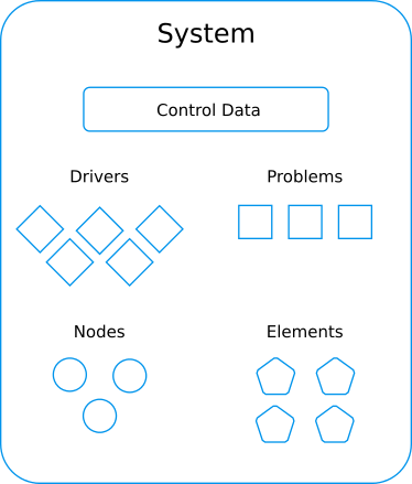
Fig. 4 MBDyn Matlab Toolbox object model.

Problems

Although Fig. 4 shows multiple problem classes, there is currently only one type of problem available, the initial-value problem. This is a problem type for solving the motion of the multibody system over time.

Nodes

Nodes come in various types, the most commonly used being structural nodes which can have 6 degrees of freedom (position and orientation), and therefore describe the kinematics of rigid-body motion in space, or 3 degrees of freedom (position) and thus describe the kinematics of point mass motion in space. All the available node types in MBDyn are:

• abstract

• electric

• hydraulic

• parameter

• structural

• thermal

Not all of these node types are currently implemented in this toolbox. Those which are are represented as Matlab classes, all ultimately derived from the mbdyn.pre.node class.

Elements

Elements are things such as forces, couples, mechanical joints and bodies which are attached to structural nodes. However, there are also a wide range of other element types avaialable in MBDyn. The full list of elements available in MBDyn is shown below:

• structural elements:

  • automatic structural

  • beam

  • body

  • couple

  • gravity

  • joint

  • joint regularization

  • plate

• aerodynamic elements:

  • aerodynamic beam2

  • aerodynamic beam3

  • aerodynamic body

  • aeromodal

  • aircraft instruments

  • air properties

  • induced velocity

• electric elements:

  • electric

• hydraulic elements:

  • hydraulic

• output elements:

  • RTAI output

  • stream output

  • stream motion output

• generic elements:

  • bind

  • bulk

  • force

  • genel

  • loadable

  • user defined

• miscellaneous element cards

Again, not every element is yet available in the Matlab toolbox. As with the nodes, those which are are represented as Matlab classes, all ultimately derived from the mbdyn.pre.element class.

Drivers

Drivers are special objects which can be required for certain configurations (see the MBDyn manual for more information). There is currently limited support for these drivers.

Control Data

Unlike the parts discussed above, control data does not refer to a class, instead this refers to general settings for the problem. These settings are accessed though properties and methods of the system class.

Example Matlab Script

The following example sets up and runs a simulation of a double pendulum. It also loads results from MBDyn output files, and plots some of them. The system to be simulated is shown in Fig. 5. This example does not demonstrate cosimulation, where forces are exchanged during simulation between Matlab and MBDyn. An example of this can be found later in this documentation.

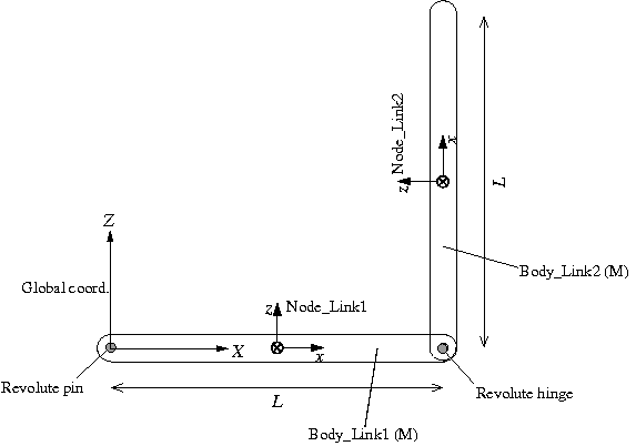
Fig. 5 Double pendulum example geometry.

The pendulum consists of two bodies. One body is attached by a pin to a fixed location. The other body is attached to the first by a hinge. A script to describe and run the problem is shown in the heavily commented listing below.

% example_double_pendulum.m
%
% this is intended to replicate the MBDyn double pendulum example which can
% be found at:
%
% http://www.sky-engin.jp/en/MBDynTutorial/chap15/chap15.html
%
% It considers a double rigid pendulum composed of two links. This example
% uses the concept of 'references' which allow one to easily set the
% relative position of the links.
%

% Let the angle between Link1 and the vertical line be theta1 and the angle
% between Link2 and Link1 be theta2, and set up some initial variables to
% hold data on the links.

% initial angle between link 1 and the vertical axis
theta1 = -pi/5;
% initial angle between link 1 and link 2
theta2 = pi/5;
% length of the links
L = 1;
% Mass or the links
M = 1;
% inertia matrix for the links
inertiamat = diag ([0., M*L^2./12., M*L^2./12.]);

% The reference class is used to assist with positioning things relative to
% known locations in the global frame. This can greatly ease the creation
% of 3D multibody models. They are also extremely useful for creating
% models in which components can be moved around while keeping the relative
% position of other components constant. 

% Create a reference object to the global orientation/location frame.
gref = mbdyn.pre.globalref ();

% Create a reference relative to the global frame, but with a different
% orientation, one rotated by theta1 radians about the y axis
ref_link1_angle = mbdyn.pre.reference ( ...
                [], ...
                mbdyn.pre.orientmat ('euler', [0, theta1, 0]), ...
                [], ...
                [], ...
                'Parent', gref, ...
                'Name', 'Ref_Link1_Angle' );


% Create a reference relative to ref_link1_angle for the location of Link
% 1's structural node. This one is at position [0.5*L; 0; 0], in the frame
% of the ref_link1_angle reference
ref_link1_node = mbdyn.pre.reference ( [0.5*L; 0; 0], ...
                                       [], ...
                                       [], ...
                                       [], ...
                                       'Parent', ref_link1_angle, ...
                                       'Name', 'Ref_Node_Link1' );

% Now create a dynamic structural node for Link 1. The global position and
% orientation of the node are taken from the ref_link1_node reference which
% converts the relative location by which it was specified into the global
% frame. 
link1node = mbdyn.pre.structuralNode6dof ( ...
                        'dynamic', ...
                        'AbsolutePosition', ref_link1_node.pos, ...
                        'AbsoluteOrientation', ref_link1_node.orientm );
            
% Create a body representing link1 which is attached to the structural node
link1 = mbdyn.pre.body (M, [], inertiamat, link1node);

% Create a reference in the frame of link 1 which points to the joint
% location between the two links
ref_link1_link2_joint = mbdyn.pre.reference ( ...
                   [L; 0; 0], ...
                   mbdyn.pre.orientmat ('euler', [0, theta2, 0]), [], ...
                   [], ...
                   'Parent', ref_link1_angle, ...
                   'Name', 'Ref_Link2');

% From the joint location create a reference to the Link 2 node
ref_link2_node = mbdyn.pre.reference ( [0.5*L; 0; 0], ...
                                       mbdyn.pre.orientmat ('orientation', eye(3)), ...
                                       [], ...
                                       [], ...
                                       'Parent', ref_link1_link2_joint, ...
                                       'Name', 'Ref_Node_Link2');

% Create structural node for link 2.
link2node = mbdyn.pre.structuralNode6dof (...
                          'dynamic', ...
                          'AbsolutePosition', ref_link2_node.pos, ...
                          'AbsoluteOrientation', ref_link2_node.orientm );

% A body for link 2 attached to link2node
link2 = mbdyn.pre.body (M, [], inertiamat, link2node);

% Next we are going to create the joints in the system, there are two
% joints, a revolute pin for link 1, and a revolute hinge between link 1
% and link 2. Both of these hinge types allow rotation around axis 3 in
% their local orientation. To get the hinges pointed in the right
% direction, therefore, we have to create an orientation which will be
% supplied to the hinges when they are created.

% Orientations can be created using the mbdyn.pre.orientmat class. This is
% essentially a wrapper for a 3x3 orientation matrix, but with various
% ways of creating it and some other useful methods, including the ability
% to draw the orientation in a figure (represented as 3 orthogonal axes).
% Here we create an orientation using the '2vectors' method. This method
% specifies an orientation by defining a plane using two non-parallel
% vectors, see the help for mbdyn.pre.orientmat for more information on
% this method. Here we create a orientatino with axis 3 pointing parallel
% to the Y-axis of the global frame
hinges_orientation = mbdyn.pre.orientmat ( ...
    '2vectors', struct ('ia', 1, 'vecA', [1;0;0], 'ib', 3, 'vecB', [0;1;0]) );

% Next create references for the location and orientation of the two
% hinges, we can make them relative to previously create references for
% convenience
ref_pin = mbdyn.pre.reference ( [], hinges_orientation, [], [], ...
                                'Parent', ref_link1_angle, ...
                                'Name', 'Ref_pin' );
                            
ref_hinge = mbdyn.pre.reference ( [], hinges_orientation, [], [], ...
                                  'Parent', ref_link1_link2_joint, ...
                                  'Name', 'Ref_hinge' );

% Create the two joint objects, first the pin joint
pinjoint = mbdyn.pre.revolutePin ( ...
                    link1node, ref_link1_angle.pos, ref_link1_angle.pos, ...
                    'NodeRelativeOrientation', ref_pin.orientm, ...
                    'PinOrientation', ref_pin.orientm );

% Next create the hinge between the two links. The revoluteHinge requires
% that you specify the location and orientation of the joint relative to
% both nodes, and these locations must match up. Although by default the
% reference frame of the location is that of the attached nodes, one can
% also force an alternative reference frame. In this case we are not
% meaning a mbdyn.pre.reference object, but rather a keyword specifying a
% particular frame. The keyword can be 'node', 'local', 'other node',
% 'other location' or 'global'. Below we explicitly specify 'node' and
% 'other node' for the location reference, and both locations are specified
% in the frame of the first structural node attached to the joint
% (which is link1node).
linkjoint = mbdyn.pre.revoluteHinge ( link1node, link2node, ...
                                      [L/2;0;0], [L/2;0;0], ...
                                      'Offset1Reference', 'node', ...
                                      'Offset2Reference', 'other node', ...
                                      'RelativeOrientation1', ref_hinge.orientm, ...
                                      'Orientation1Reference', 'global', ...
                                      'RelativeOrientation2', ref_hinge.orientm, ...
                                      'Orientation2Reference', 'global' ...
                                    );
                                
% Finally, create a gravity object. The default setting produce a uniform
% gravitational field directed along the negative z asis. More advanced
% forms of gravitational field are possible
gravity = mbdyn.pre.gravity();

% The double pendulum system is now fully described and we can set up the
% problem settings
prb = mbdyn.pre.initialValueProblem (0, 10, 1e-3, ...
                                     'ResidualTolerance', 1e-9);


% To solve the system, we create an mbdyn.pre.system object, into which we
% put all the nodes and elements and the problem object. In this case we
% also supply some references. This is optional and they are not used for
% the solution of the problem. They are used only for visualisation
% purposes (as will be be seen in the section below)
mbsys = mbdyn.pre.system ( {prb}, ...
                           'Nodes', {link1node, link2node}, ...
                           'Elements', { link1, link2, pinjoint, ...
                                         linkjoint, gravity }, ...
                           'References', { ref_link1_angle, ...
                                           ref_link1_node,  ...
                                           ref_link1_link2_joint,  ...
                                           ref_link2_node,  ...
                                           ref_pin,  ...
                                           ref_hinge }, ...
                           'DefaultOrientation', 'orientation matrix');

%% Visualisation of the system
%
% To assist with model development, various visualisation tools are
% provided so one can check and debug the orientations and locations of
% components
%

% Below we set the size of nodes and size and color of the bodies for
% visualisation purposes. This has no effect on the simulation. By default
% bodies are represented as simple box shapes. Below we are simply changing
% the shape of these boxes. It is also possible to specify STL files for
% bodies, in which case the STL mesh shape will insead be used in the
% visualisation.
%
% Note that it is possible to do this *after* inserting them into the
% system as they are derived from the Matlab handle class. This means
% changes to these objects will be propogated to the copies in the system
% (or elsewhere). This is something to bear in mind for all the mbdyn
% classes, as nearly all are derived from the handle class.
%
mbsys.setStructuralNodeSize (L/10, L/10, L/10);
link1.setSize (L, L/10, L/10);
link2.setSize (L, L/10, L/10);
link1.setColour ('r');
link1.setColour ('b');
% pinjoint.setSize (L/10, L/10, L/10);
pinjoint.setColour ('k');
% linkjoint.setSize (L/10, L/10, L/10);
linkjoint.setColour ('g');

% Draw the system to check it is set up correctly, we turn on plotting of
% the supplied reference objects, as by default they are not plotted.
mbsys.draw ( 'Mode', 'wireghost', ...
             'References', true, ...
             'ReferenceScale', 0.5, ...
             'AxLims', [-2, 2; -2, 2; -2, 2;] );

%% Run MBDyn For Problem
%
% Now we can actually generate the the input file for the MBDyn program,
% and run it to solve the problem

inputfile = 'example_double_pendulum.mbd';

% Generate the input file for MBDyn in the specified location
mbsys.generateMBDynInputFile (inputfile);

% Start mbdyn with the generated input file using the start_mbdyn function
% from the mbdyn.mint package. Note this is different from the mbdyn.pre
% package all the previous classes were from. mint is short for
% m-interface.
mbdyn.mint.start_mbdyn (inputfile);

%% Post-processing
%
% A class is also provided to post-process and visualise the results of an
% MBDyn simulation

% Load data into post-processing object, the ouput files are by default
% created by MBDyn in the same location as the input files but with
% alternative file extensions. We supply the input file, meaning the
% postproc class looks for output files of the same name and location, but
% with different file extensions
mbdynpost = mbdyn.postproc (inputfile, mbsys);

% Plot node trajectories
mbdynpost.plotNodeTrajectories ();

% Make a 2D plot of the node positions
mbdynpost.plotNodePositions ();

% Make a 2D plot of the node velocities
mbdynpost.plotNodeVelocities ();

% Make a 2D plot of the node angular velocities
mbdynpost.plotNodeAngularVelocities ();

% Plot a particular time step of interest
mbdynpost.drawStep (500, ...
    'AxLims', [-2, 2; -0.5, 0.5;  -2, 1]);

% Animate the entire simulation, saving it in an avi file
mbdynpost.animate ( 'PlotTrajectories', true, ...
                    'DrawLabels', true, ...
                    'Skip', 20, ...
                    'DrawMode', 'solid', ...
                    'Light', true, ...
                    'AxLims', [-2, 2; -0.5, 0.5;  -2, 1], ...
                    'VideoFile', 'example_double_pendulum.avi');
                
                

When run, the script ultimately produces six figures shown below. Fig. 6 shows the system with it’s initial setup, produced using the mbdyn.pre.system.draw () method. The remaining fgures, Fig. 7, Fig. 8, Fig. 9, Fig. 10, and Fig. 11 all show results from the simulation and produced using the mbdyn.postproc class.

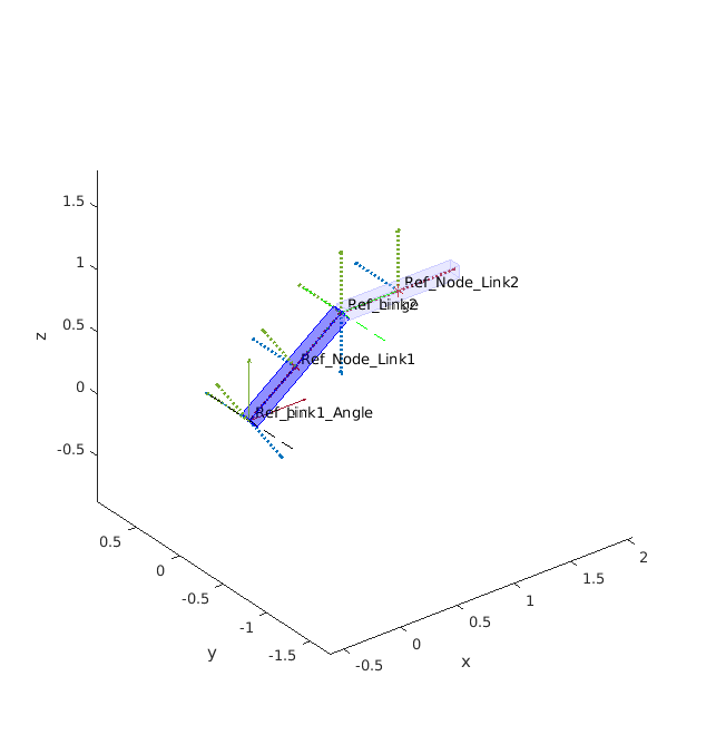
Fig. 6 Double pendulum initial setup.

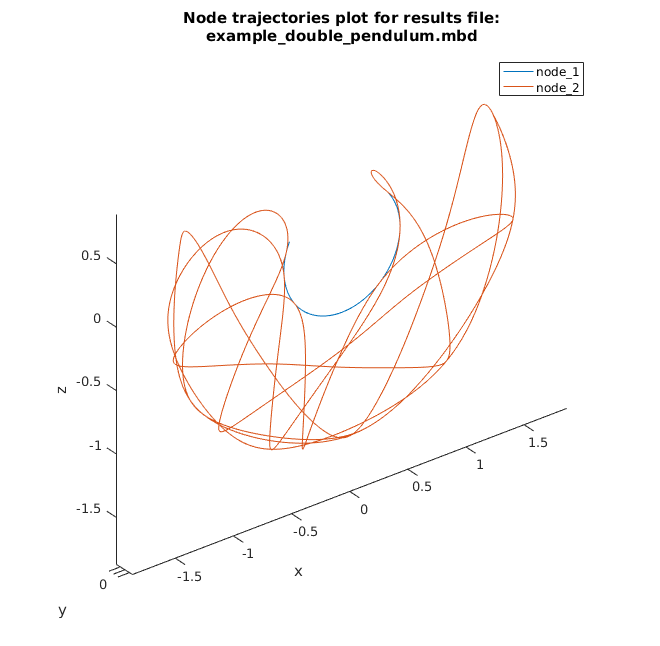
Fig. 7 Double pendulum result plot.

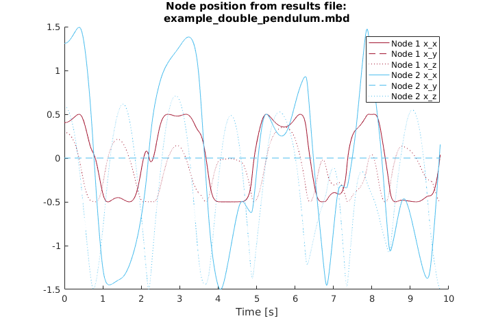
Fig. 8 Double pendulum result plot.

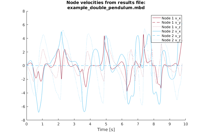
Fig. 9 Double pendulum result plot.

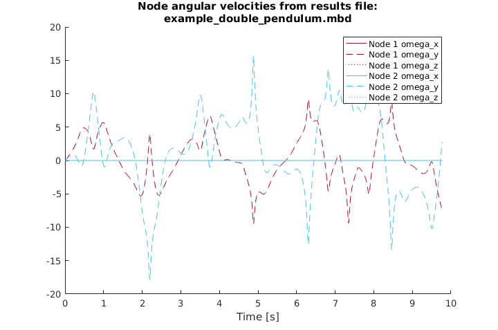
Fig. 10 Double pendulum result plot.

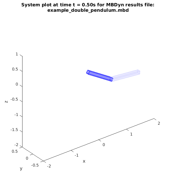
Fig. 11 Double pendulum result plot.

The final command in the example, i.e.

% Animate the entire simulation, saving it in an avi file
mbdynpost.animate ( 'PlotTrajectories', true, ...
                    'DrawLabels', true, ...
                    'Skip', 20, ...
                    'DrawMode', 'solid', ...
                    'Light', true, ...
                    'AxLims', [-2, 2; -0.5, 0.5;  -2, 1], ...
                    'VideoFile', 'example_double_pendulum.avi');
                
                

Animates the simulation in a figure and saves the animation to an avi file, the video can be seen below:

Getting Help

In general the mbdyn toolbox classes are documented (although this is an ongoing project), so to learn more about a class one can use the matlab built-in help and doc commands. e.g.:

help mbdyn.pre.reference

An API reference containing the same information (actually generated from the help for the classes) is provided with this docuement.