Cosimulation
The previous examle simply set up a simulation and ran it, with not input from Matlab during the solving process. MBDyn is also capable of cosimulation with external software. This allows forces to be sent to MBDyn based on kinematics sent by MBDyn to the external software. The MBDyn Matlab toolbox includes tools to assist with connecting to an MBDyn simulation and sending forces as the simulation progresses. Here we will demonstrate the use of these tools with a simple example.
The cosimulation process is primarily handled by the
mbdyn.mint.MBCNodal class which manages the communication with
MBDyn. The mbdyn.mint namespace holds all of the functions or
classes specifically related to cosimulation.
mbdyn.mint.MBCNodal is used to start the mbdyn executeable, set
up communication to it, and has various methods to then get and send
appropriate data at each time step between Matlab and MBDyn. It will
also close communication and quit MBDyn in the event that the
simulation is to be ended. mbdyn.mint.MBCNodal is uesed in
tandem with the mbdyn.pre.externalStructuralForce element which
adds an element to the MBDyn input file which tells MBDyn what data
to expect from Matlab. How this works is best demonstrated with an
example.
Cosimulation Example
A simple example of cosimulation is presented in the listing below, which simulates a small solid sphere, in a gravitational field, which has some additional forces applied to it during the simulation which are supplied by Matlab. The position and velocity are also read by Matlab as the simulation progesses.
  1%% example_basic_cosimulation.m
  2%
  3%
  4% Make a very simple problem of a single body (a sphere) in a uniform
  5% gravitational field. Apply a force after some time, then turn it off
  6% after some more time
  7
  8%% Problem Definition
  9
 10% define the sphere
 11mass = 1;
 12radius = 0.05;
 13inertiamat = eye (3) * (2/5) * mass * radius^2;
 14
 15% sim start time
 16itime = 0;
 17% sim end time
 18ftime = 10;
 19% sim time step
 20nsteps = 100;
 21tstep = (ftime - itime) / nsteps;
 22
 23% set aceleration due to gravity
 24g = 9.81;
 25
 26% size of force to apply to the sphere
 27force_magnitude = 2 * mass * g;
 28% angle of applied force in the X-Z plane
 29force_angle = deg2rad (45);
 30% time when to start applying the force
 31force_start_time = itime + 0.1 * (ftime - itime);
 32% time when to stop applying the force
 33force_stop_time = itime + 0.75 * (ftime - itime);
 34
 35% now make the MBDyn system
 36
 37% create a dynamic node at the origin
 38node = mbdyn.pre.structuralNode6dof ('dynamic');
 39
 40% create the body attached to the node
 41cog = [0;0;0];
 42body = mbdyn.pre.body (mass, cog, inertiamat, node);
 43
 44% add gravity
 45grav = mbdyn.pre.gravity ('GravityAcceleration', g);
 46
 47% set up the communication methods between MBDyn and Matlab
 48if ispc
 49    % windows does not have 'local' sockets like Linux, so use inet socket
 50    communicator = mbdyn.pre.socketCommunicator ('Port', 5500, ...
 51                                                 'Coupling', 'tight', ...
 52                                                 'Create', 'yes', ...
 53                                                 'SleepTime', 0, ...
 54                                                 'SendAfterPredict', 'no');
 55else
 56    % add the socket forces
 57    communicator = mbdyn.pre.socketCommunicator ('Path', '/tmp/mbdyn.sock', ...
 58                                                 'Coupling', 'tight', ...
 59                                                 'Create', 'yes', ...
 60                                                 'SleepTime', 0, ...
 61                                                 'SendAfterPredict', 'no');
 62end
 63
 64% create the external force element
 65matlab_force = mbdyn.pre.externalStructuralForce ({node}, [], communicator);
 66
 67% set up the initial-value problem
 68pbm = mbdyn.pre.initialValueProblem ( itime, ftime, tstep, ...
 69                                      'MaxIterations', 10, ...
 70                                      'ResidualTolerance', 1e-9 );
 71
 72% put it all together in an MBDyn system
 73mbsys = mbdyn.pre.system ( pbm, ...
 74                           'Nodes', {node}, ...
 75                           'Elements', {body, grav, matlab_force}, ...
 76                           'DefaultOrientation', 'orientation matrix' );
 77
 78%% Start MBDyn
 79
 80% put MBDyn input file in temporary directory, we don't need it once MBDyn
 81% has read it
 82mbdpath = fullfile (tempdir(), 'example_cosim.mbd' );
 83
 84% put output in new folder in current directory
 85outputdir = fullfile ('.', 'Test_mbdyn_MBCNodal_output');
 86
 87mkdir (outputdir);
 88
 89% make output file be named Test_mbdyn_MBCNodal.mov etc. in the output
 90% directory
 91outputfile_prefix = fullfile (outputdir, 'Test_mbdyn_MBCNodal');
 92
 93% create the MBCNodal object to handle communication with MBDyn
 94mb = mbdyn.mint.MBCNodal ('MBDynPreProc', mbsys, ...
 95                          'UseMoments', true, ...
 96                          'MBDynInputFile', mbdpath, ...
 97                          'OverwriteInputFile', true, ...
 98                          'OutputPrefix', outputfile_prefix ...
 99                          );
100
101mb.start ('Verbosity', 1);
102
103nnodes = mb.GetNodes ();
104
105%% Perform Simulation Loop
106
107% to match example program
108maxiter = 3;
109
110% initialise some variables
111status = 0;
112time = 0;
113ind = 1;
114pos = zeros (3,1);
115rot = zeros (3,3,1);
116
117while status == 0
118
119    % Apply the force depending on the specified start and end times
120    if time(ind) < force_start_time
121        fmag = 0;
122    elseif time(ind) >= force_stop_time
123        fmag = 0;
124    else
125        fmag = force_magnitude;
126    end
127
128    % Make 3D force vector to apply to node
129    forces = [ fmag * cos(force_angle);
130               0;
131               fmag * sin(force_angle); ];
132
133    for iter = (maxiter-1):-1:1
134
135        status = mb.GetMotion ();
136
137        if status ~= 0
138            break;
139        end
140
141        fprintf (1, 'iter: %d, iterstatus: %d\n', iter, status);
142
143        % set the forces
144        mb.F (forces);
145        mb.M (zeros (3,1));
146
147        % apply the force but tell MBDyn that the simulation at the Matlab end
148        % has not converged, so it cannot proceed to the next time step, but
149        % should recalculate the motion based on the new forces and resend
150        % the result back to the Matlab simulation.
151        mb.applyForcesAndMoments (false)
152
153    end
154
155    if status ~= 0
156        break;
157    end
158
159    status = mb.GetMotion ();
160
161    if status ~= 0
162        break;
163    end
164
165    pos(:,ind) = mb.X(1);
166
167    rot(:,:,ind) = mb.GetRot();
168
169    % set the forces
170    mb.F (forces);
171    mb.M (zeros (3,1));
172
173    % apply the force and tell MBDyn that the simulation at the Matlab end
174    % has converged, so it can proceed to the next time step
175    mb.applyForcesAndMoments (true)
176
177    % get next time step
178    ind = ind + 1;
179    time(ind) = time(ind-1) + tstep;
180
181end
182
183clear mb;
184
185% strip the extra time step which will have been added
186time(end) = [];
187
188%% Perform Post-Processing
189
190% we can plot the local Matlab data as normal
191plot ( time, pos');
192legend ('x position', 'y position', 'z position');
193xlabel ('time [s]');
194ylabel ('displacement [m]');
195
196% load the results files
197mbout = mbdyn.postproc ( outputfile_prefix, mbsys );
198
199% plot the node trajectory, we replace the default title with our own
200mbout.plotNodeTrajectories ('Title', 'Sphere Trajectory');
201
202% plot all the node velocities
203mbout.plotNodeVelocities ()
This produces the plots in Fig. 12, Fig. 13 and Fig. 14.
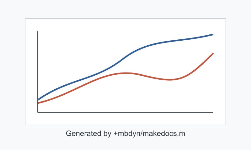
Fig. 12 Basic cosimulation result plot.
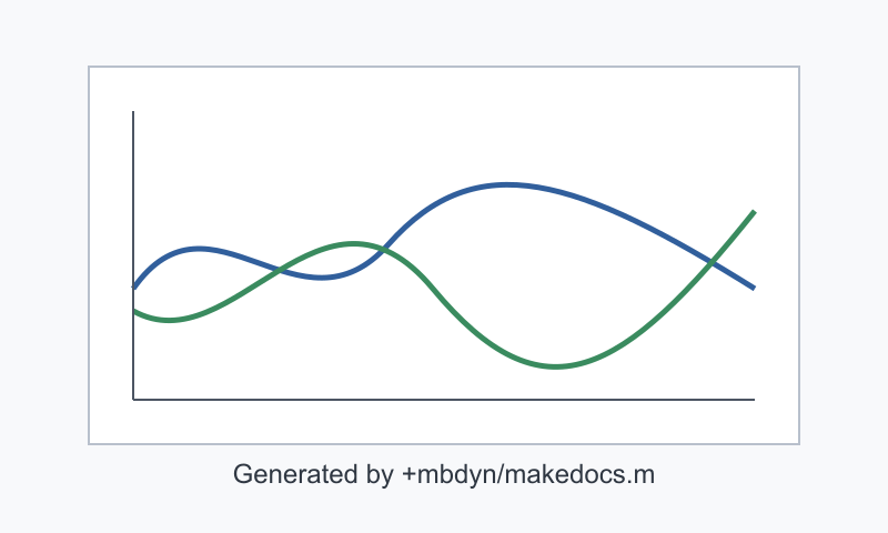
Fig. 13 Basic cosimulation result plot.
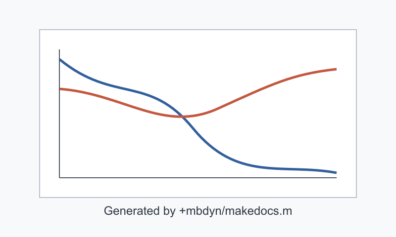
Fig. 14 Basic cosimulation result plot.
We can take a closer look at the various parts of this example in order to fully understand it.
The first part of the file sets up the MBDyn problem, which is solving the motion of a sphere with some forces applied to it, and the first section of this part, shown below, is just setting up some things that are all handled internally by MBDyn. That is, the node, the body and gravity.
% define the sphere
mass = 1;
radius = 0.05;
inertiamat = eye (3) * (2/5) * mass * radius^2;

% sim start time
itime = 0;
% sim end time
ftime = 10;
% sim time step
nsteps = 100;
tstep = (ftime - itime) / nsteps;

% set aceleration due to gravity
g = 9.81;

% size of force to apply to the sphere
force_magnitude = 2 * mass * g;
% angle of applied force in the X-Z plane
force_angle = deg2rad (45);
% time when to start applying the force
force_start_time = itime + 0.1 * (ftime - itime);
% time when to stop applying the force
force_stop_time = itime + 0.75 * (ftime - itime);

% now make the MBDyn system

% create a dynamic node at the origin
node = mbdyn.pre.structuralNode6dof ('dynamic');

% create the body attached to the node
cog = [0;0;0];
body = mbdyn.pre.body (mass, cog, inertiamat, node);

% add gravity
grav = mbdyn.pre.gravity ('GravityAcceleration', g);
The next part is adding elements which MBDyn uses to communicate
with Matlab (or any external solver). The
externalStructuralForce element tells MBDyn about which nodes
are going to have forces applied by the external solver, and a few
other things about the nature of those forces. The
socketCommunicator tells MBDyn how the communication with the
external solver will be performed, other communication methods are
possible.
% set up the communication methods between MBDyn and Matlab
if ispc
    % windows does not have 'local' sockets like Linux, so use inet socket
    communicator = mbdyn.pre.socketCommunicator ('Port', 5500, ...
                                                 'Coupling', 'tight', ...
                                                 'Create', 'yes', ...
                                                 'SleepTime', 0, ...
                                                 'SendAfterPredict', 'no');
else
    % add the socket forces
    communicator = mbdyn.pre.socketCommunicator ('Path', '/tmp/mbdyn.sock', ...
                                                 'Coupling', 'tight', ...
                                                 'Create', 'yes', ...
                                                 'SleepTime', 0, ...
                                                 'SendAfterPredict', 'no');
end

% create the external force element
matlab_force = mbdyn.pre.externalStructuralForce ({node}, [], communicator);
The usual problem and system set up follows.
pbm = mbdyn.pre.initialValueProblem ( itime, ftime, tstep, ...
                                      'MaxIterations', 10, ...
                                      'ResidualTolerance', 1e-9 );

% put it all together in an MBDyn system
mbsys = mbdyn.pre.system ( pbm, ...
                           'Nodes', {node}, ...
                           'Elements', {body, grav, matlab_force}, ...
                           'DefaultOrientation', 'orientation matrix' );
Following this is a section where the instantiation of the
mbdyn.mint.MBCNodal object takes place. The MBCNodal class handles
both the starting up of the MBDyn program, and also the initiation
of communication between Matlab and MBDyn. If an
mbdyn.pre.system object is passed to MBCNodal, it will
discover the details of the chosen communication method and settings
from this. However, it is not necessary to use an
mbdyn.pre.system object, and communication can be set up
manually, if, say, one were using a predefined MBDyn input file, and
not generating file using the Matlab preprocessor. However, this
method ensures a change to the communication method or nodes for
which forces are to be applied etc. are automatically propogated to
the MBCNodal object and everything is more easily kept up to
date if the problem is modified or expanded.
%% Start MBDyn

% put MBDyn input file in temporary directory, we don't need it once MBDyn
% has read it
mbdpath = fullfile (tempdir(), 'example_cosim.mbd' );

% put output in new folder in current directory
outputdir = fullfile ('.', 'Test_mbdyn_MBCNodal_output');

mkdir (outputdir);

% make output file be named Test_mbdyn_MBCNodal.mov etc. in the output
% directory
outputfile_prefix = fullfile (outputdir, 'Test_mbdyn_MBCNodal');

% create the MBCNodal object to handle communication with MBDyn
mb = mbdyn.mint.MBCNodal ('MBDynPreProc', mbsys, ...
                          'UseMoments', true, ...
                          'MBDynInputFile', mbdpath, ...
                          'OverwriteInputFile', true, ...
                          'OutputPrefix', outputfile_prefix ...
                          );

mb.start ('Verbosity', 1);

nnodes = mb.GetNodes ();
By default MBCNodal searches for the MBDyn executable in some
standard install locations. If your version of MBDyn is not in these
locations (e.g. you compiled it yourself) you can poiont MBDyn to a
specific place. See the help for the mbdyn.mint.MBCNodal
constructor to see all the options that can be sued when creating
the object.
The following part is the main simulation loop. In this loop forces and positions are exchanged with MBDyn until the simulation is finished.
%% Perform Simulation Loop

% to match example program
maxiter = 3;

% initialise some variables
status = 0;
time = 0;
ind = 1;
pos = zeros (3,1);
rot = zeros (3,3,1);

while status == 0

    % Apply the force depending on the specified start and end times
    if time(ind) < force_start_time
        fmag = 0;
    elseif time(ind) >= force_stop_time
        fmag = 0;
    else
        fmag = force_magnitude;
    end

    % Make 3D force vector to apply to node
    forces = [ fmag * cos(force_angle);
               0;
               fmag * sin(force_angle); ];

    for iter = (maxiter-1):-1:1

        status = mb.GetMotion ();

        if status ~= 0
            break;
        end

        fprintf (1, 'iter: %d, iterstatus: %d\n', iter, status);

        % set the forces
        mb.F (forces);
        mb.M (zeros (3,1));

        % apply the force but tell MBDyn that the simulation at the Matlab end
        % has not converged, so it cannot proceed to the next time step, but
        % should recalculate the motion based on the new forces and resend
        % the result back to the Matlab simulation.
        mb.applyForcesAndMoments (false)

    end

    if status ~= 0
        break;
    end

    status = mb.GetMotion ();

    if status ~= 0
        break;
    end

    pos(:,ind) = mb.X(1);

    rot(:,:,ind) = mb.GetRot();

    % set the forces
    mb.F (forces);
    mb.M (zeros (3,1));

    % apply the force and tell MBDyn that the simulation at the Matlab end
    % has converged, so it can proceed to the next time step
    mb.applyForcesAndMoments (true)

    % get next time step
    ind = ind + 1;
    time(ind) = time(ind-1) + tstep;

end

clear mb;

% strip the extra time step which will have been added
time(end) = [];
In this loop we are faking the Matlab solving algorithm’s
convergence by adding in fake iterations. In a real simulation, you
would use this mechanism to alow then MBDyn solution and force
calulation to converge together when the calculated forces depended
on the motion. In the example, they don’t, so we could have skipped
the iterations and just sent the forces. If the forces really don’t
depend very much on the motion, it is also possible to define the
communication between the solver and MBDyn as ‘loose’ (rather than
‘tight’) when setting up the communicator object for the problem.
When ‘loose’ is used, the convergence flag passed in to
applyForcesAndMoments is ignored, and the MBDyn simulation
always steps forward using the supplied forces.
The rest of the file, shown below, demonstrates how to use the post-processing class to examine the results from output files produced by MBDyn.
%% Perform Post-Processing

% we can plot the local Matlab data as normal
plot ( time, pos');
legend ('x position', 'y position', 'z position');
xlabel ('time [s]');
ylabel ('displacement [m]');

% load the results files
mbout = mbdyn.postproc ( outputfile_prefix, mbsys );

% plot the node trajectory, we replace the default title with our own
mbout.plotNodeTrajectories ('Title', 'Sphere Trajectory');

% plot all the node velocities
mbout.plotNodeVelocities ()
This works in exactly the same way as for the non-cosimulation case,
however, it is worth noting that since Matlab is able to extract and
store data from the simulation as it progresses, this might be
redundant. In this case, one can use the ‘DefaultOutput’ option of
the mbdyn.pre.system class to turn off all output logging to
files by setting it to ‘none’. See the help for the system class for
more information.
Helper Classes
Two other classes are provided to assist with the application of
forces, mbdyn.mint.twoNodeTranslationalForce and
mbdyn.mint.twoNodeTorque. These classes assist with the
application of forces in the correct frame of reference. For
instance, mbdyn.mint.twoNodeTranslationalForce might be used
when modelling an actuator of some kind which is movng and changing
orientation in the global frame.
mbdyn.mint.twoNodeTranslationalForce has methods to calculate
the relative displacement and velocity of the two nodes to which it
is linked in a direction parallel to one axis of one of the nodes.
It can then be used to apply forces to both nodes, also parallel to
this axis and then transform these forces to forces in the global
frame suitable for application using the MBDyn external structural
force element (which expects forces in the global frame).