NEMOH
The time domain simulator requires that you supply frequency domain hydrodynamic coefficients derived from potential flow analysis. One program capable of generating the required data is NEMOH. NEMOH is a Boundary Element Methods (BEM) code dedicated to the computation of first order wave loads on offshore structures (added mass, radiation damping, diffraction forces). It was been developed by researchers at Ecole Centrale de Nantes for 30 years before being released under a free software licence (Apache v2).
Detailed information can be found at the project homepage linked above and in academic papers, links for which can also be found at the project homepage. This document focusses on the use of a Matlab preprocessor which has been developed as part of the EWST to ease the creation of this data for WECs, rather than the details of what NEMOH produces.
Getting Nemoh
For information and instructions on obtaining and installing Nemoh, see Nemoh. Note also the section The NEMOH Executables Location below.
NEMOH Preprocessor
The Matlab preprocessor for NEMOH is based on an object oriented
approach. Two classes are used to describe the system to be simulated
a body class and a system class. The system class acts as a
container for one or more body objects and generates the Nemoh input
files. Like the EWST, and MBDyn tools, the NEMOH classes are intended
to be a standalone package and as such are in their own namespace nemoh.
This means the classes must be referenced using syntax like nemoh.body
and nemoh.system. The use of the preprocessor is best demonstrated
with a simple example, as shown in the listing below, which shows how to
simulate a simple cylinder using the NEMOH preprocessor.
1 2 3 4 5 6 7 8 9 10 11 12 13 14 15 16 17 18 19 20 21 22 23 24 25 26 27 28 29 30 31 32 33 34 35 36 37 38 39 40 41 42 43 44 45 46 47 48 49 50 51 52 53 54 55 56 57 58 59 60 61 62 63 64 65 66 67 68 69 70 71 72 73 74 75 76 77 78 79 80 81 82 83 84 85 86 87 88 89 90 91 92 93 94 95 96 97 98 99 100 101 102 103 104 105 106 107 108 109 110 111 112 113 114 115 116 117 118 119 120 121 122 123 124 125 126 127 | % example_nemoh_cylinder.m
%
% Example file for nemoh package generating a basic cylinder
%
%
dir = fileparts ( which ('example_nemoh_cylinder') );
inputdir = fullfile (dir, 'example_nemoh_cylinder_output');
%% create the Nemoh body
% create a body object which will be the cylinder
cylinder = nemoh.body (inputdir);
radius = 5; % Radius of the cylinder
draft = -10; % Height of the submerged part
r = [radius radius 0];
z = [0 draft draft];
ntheta = 30;
verticalCentreOfGravity = -2;
% The body shape is defined using a 2D profile rotated around the z axis,
% created using the makeAxiSymmetricMesh method. The nemoh.body object
% actually has a makeCylinderMesh method which we could use to create such
% a mesh, but the makeAxiSymmetricMesh method is used here just for
% demonstration of the capability. There is also a makeSphereMesh method,
% other basic shapes may be introduced in the future. Existing NEMOH meshes
% can be imported, and also STL files.
cylinder.makeAxiSymmetricMesh (r, z, ntheta, verticalCentreOfGravity);
%% draw the course body mesh (will be refined later)
cylinder.drawMesh ();
axis equal;
%% Create the nemoh simulation
% here we insert the cylinder body at creation of the simulation, but could
% also have done this later by calling addBody
sim = nemoh.simulation ( inputdir, ...
'Bodies', cylinder );
%% write mesh files
% write mesh file for all bodies (just one in this case)
sim.writeMesherInputFiles ();
%% process mesh files
% process mesh files for all bodies to make ready for Nemoh
sim.processMeshes ();
%% Draw all meshes in one figure
sim.drawMesh ();
axis equal;
%% Generate the Nemoh input file
% generate the file for 10 frequencies in the range defined by waves with
% periods from 10s to 3s.
T = [10, 3];
sim.writeNemoh ( 'NWaveFreqs', 10, ...
'MinMaxWaveFreqs', 2 * pi() * (1./T) );
% The above code demonstrates the use of optional arguments to writeNemoh
% to set the desired wave frequencies. If the wave frequencies were not
% specified a default value would be used. These are not the only possible
% options for writeNemoh. The following optional arguments are available,
% and the defaults used if they are not supplied are also shown:
%
% DoIRFCalculation = true;
% IRFTimeStep = 0.1;
% IRFDuration = 10;
% NWaveFreqs = 1;
% MinMaxWaveFreqs = [0.8, 0.8];
% NDirectionAngles = 1;
% MinMaxDirectionAngles = [0, 0];
% FreeSurfacePoints = [0, 50];
% DomainSize = [400, 400];
% WaterDepth = 0;
% WaveMeasurementPoint = [0, 0];
%
% For more information on these arguments, see the help for the writeNemoh
% method.
%% Run Nemoh on the input files
% The run Method invokes the Nemo programs on the generated input files.
% Before running it also first generates the ID.dat file and input.txt file
% for the problem. See the Nemoh documentation for more information about
% these files. After generating the files, the preprocessor, solver and
% postprocessor are all run on the input files in sequence.
%
sim.run ()
% Other options supported by the run Method, but not used above are:
%
% 'Solver' - integer or string. Used to select the solver for
% the problem, the following values are possible:
%
% 0 or 'direct gauss' or 'directgauss'
% 1 or 'GMRES'
% 2 or 'GMRES-FHM' or 'GMRES with FHM'
%
% The string forms are case-insensitive (e.g. 'gmres' works
% just as well as 'GMRES'.
%
% 'SavePotential' - logical (true/false) flag indicating whther
% the potential should be saved for visualisation.
%
% 'GMRESRestart' - scalar integer. Restart criteria for the
% gmres solver types. Ignored for other solvers. Default is
% 20.
%
% 'GMRESTol' - scalar value. Tolerance for the gmres solver
% types. Ignored for other solvers. Default is 5e-7.
%
% 'GMRESMaxIterations' - scalar integer. Maximum number of
% iterations allowed for the gmres solver types. Ignored for
% other solvers. Default is 100.
%
% 'Verbose' - logical (true/false) flag determning whether to
% display some text on the command line informing on the
% progress of the simulation.
|
This script can be broken down as follows. The fist section simply does some Matlab magic to locate the directory containing the example file, and create a subdirectory in that directory in which we will generate the NEMOH input files from the Matlab description of the problem
% example_nemoh_cylinder.m
%
% Example file for nemoh package generating a basic cylinder
%
%

dir = fileparts ( which ('example_nemoh_cylinder') );

inputdir = fullfile (dir, 'example_nemoh_cylinder_output');
The next part creates the body for for which the hydrodynamics will be
solved. A simulation can be made up of multiple bodies, but here we will
just have the cylinder. In this case, the cylinder is specified using a 2D
profile from which a 3D mesh is generated by rotating it around the Z axis.
The method makeAxiSymmetricMesh is provided to accomplish this. See
the help for makeAxiSymmetricMesh for more details on how to specify
a mesh in this way.
Note also the use nemoh package namespace in the body creation command.
%% create the Nemoh body

% create a body object which will be the cylinder
cylinder = nemoh.body (inputdir);

radius = 5; % Radius of the cylinder
draft = -10; % Height of the submerged part
r = [radius  radius  0];
z = [0       draft   draft];
ntheta = 30;
verticalCentreOfGravity = -2;

% The body shape is defined using a 2D profile rotated around the z axis,
% created using the makeAxiSymmetricMesh method. The nemoh.body object
% actually has a makeCylinderMesh method which we could use to create such
% a mesh, but the makeAxiSymmetricMesh method is used here just for
% demonstration of the capability. There is also a makeSphereMesh method,
% other basic shapes may be introduced in the future. Existing NEMOH meshes
% can be imported, and also STL files.
cylinder.makeAxiSymmetricMesh (r, z, ntheta, verticalCentreOfGravity);
makeAxiSymmetricMesh creates only a course representation of the mesh,
which must be refined by the Nemoh meshing program. However, at this point
we can draw the course mesh by calling the drawMesh method.
%% draw the course body mesh (will be refined later)

cylinder.drawMesh ();
axis equal;
The mesh is shown in Fig. 9:
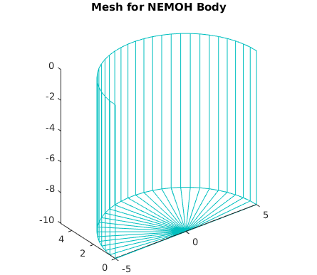
As can be seen, by default the symmetry of the body is taken advantage of to reduce the computation time by calculating for only half the axisymmetric mesh.
The next section creates a NEMOH simulation preprocessor object and puts the body into it at the same time.
%% Create the nemoh simulation

% here we insert the cylinder body at creation of the simulation, but could
% also have done this later by calling addBody
sim = nemoh.simulation ( inputdir, ...
                         'Bodies', cylinder );
Bodies don’t have to added at this point, they can be also be added by calling
the nemoh.simulation.addBody method later, the ‘Bodies’ argument is optional.
The simulation has one non-optional argument, which is the input directory where
all NEMOH files will be generated.
The nest step writes mesh files for each of the bodies in the simulation (just
the cylinder in this case). This method calls the writeMesh method for each
body in the simulation.
%% write mesh files

% write mesh file for all bodies (just one in this case)
sim.writeMesherInputFiles ();
What is actually done by writeMesh depends on the type of mesh the body has.
For the axisymmetric mesh type it writes the course mesh description in a file
format understood by the NEMOH meshing program. The mesh program must be run
on the course mesh input file to generate the mesh file suitable for input to
the other NEMOH programs. To do this step, the processMeshes method is called.
%% process mesh files

% process mesh files for all bodies to make ready for Nemoh
sim.processMeshes ();
processMeshes calls the processMesh method for every body in the
simulation. processMesh does any processing required for the body mesh to
create the appropriate input files for the other NEMOH programs. What this
processing actually is (if any) depends on the mesh type.
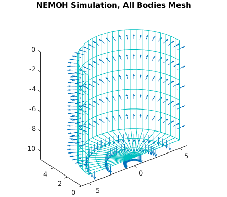
With the mesh files generated, we can draw the meshes again:
%% Draw all meshes in one figure

sim.drawMesh ();
axis equal;
The simulation drawMesh object draws the meshes for all bodies in the
simulation in one figure. The now refined cylinder mesh is shown in
Fig. 10. The blue arrows in the figure denote
the direction of the mesh face normals. NEMOH requires that these point
outward into the fluid.
We can now proceed to generate the Nemoh input files. It is at this point that the simulation parameters are provided.
%% Generate the Nemoh input file

% generate the file for 10 frequencies in the range defined by waves with
% periods from 10s to 3s.
T = [10, 3];

sim.writeNemoh ( 'NWaveFreqs', 10, ...
                 'MinMaxWaveFreqs', 2 * pi() *  (1./T) );

% The above code demonstrates the use of optional arguments to writeNemoh
% to set the desired wave frequencies. If the wave frequencies were not
% specified a default value would be used. These are not the only possible
% options for writeNemoh. The following optional arguments are available,
% and the defaults used if they are not supplied are also shown:
%
% DoIRFCalculation = true;
% IRFTimeStep = 0.1;
% IRFDuration = 10;
% NWaveFreqs = 1;
% MinMaxWaveFreqs = [0.8, 0.8];
% NDirectionAngles = 1;
% MinMaxDirectionAngles = [0, 0];
% FreeSurfacePoints = [0, 50];
% DomainSize = [400, 400];
% WaterDepth = 0;
% WaveMeasurementPoint = [0, 0];
%
% For more information on these arguments, see the help for the writeNemoh
% method.
As stated in the comments in the code section above, there are several optional
arguments which can be provided to control the calculation, and details about
their use can be found in the help text for the nemoh.simulation/writeNemoh
method. This help is shown below:
Output of help nemoh.simulation/writeNemoh
  generates the Nemoh.cal input file for NEMOH

  Syntax

  writeNemoh (ns)
  writeNemoh (ns, 'Parameter', value)

  Description

  writeNemoh generates the Nemoh.cal input file for the NEMOH
  BEM solver programs.

  Input

   ns - nemoh.simulation object

  Additional optional arguments may be supplied as
  parameter-value pairs. The available options are:

   'DoIRFCalculation' - logical (true/false) flag determining
     whether the impulse response function for the radiation
     force is calculated. Default is true if not supplied.

   'IRFTimeStep' - Scalar time step in seconds to be used for
     the IRF calcualtion. Default is 0.1 if not supplied.

   'IRFDuration' - Scalar duration in seconds for the IRF
     calculation. Default is 10 if not supplied.

   'NWaveFreqs' - Scalar integer number of wave frequencies for
     which to calculate the hydrodynamic date. Default is 1 if
     not supplied.

   'MinMaxWaveFreqs' - If NWaveFreqs is set to 1, this is a
     scalar value, the wave frequency at which to do the
     simulation, in this case a two element vector with both
     values the same is also acceptable. If NWaveFreqs > 1,
     this must be a two element vector containing the min and
     max values of the frequency range to be computed. Default
     is 0.8 if not supplied.

   'NDirectionAngles' - Number of directions to be used to
     calculate the Kochin function. Default is 0 if not
     supplied, meaning no Kochin function calculation is
     performed.

   'MinMaxDirectionAngles' - Two element vector containing the
     min and max angles for the Kochin function calculation.
     Default is 0 if not supplied.

   'FreeSurfacePoints' - Two element vector containing the
     number of points at which to calcualte the free surface
     elevation. The first element is the number of points in
     the x direction (0 for no calculations) and y direction
     By default no calculations are performed (the default
     value used to set the input in Nemoh.cal is [0,50]).

   'DomainSize' - Two element vector containing the domain size
     in the x and y direction. Default is [400, 400] if not
     supplied.

   'WaterDepth' - Scalar value of the water depth, a value of 0
     means infinite depth. Default is 0 if not supplied.

   'WaveMeasurementPoint' - Two element vector containing the
     wave measurement point [XEFF YEFF]. Default is [0, 0] if
     not supplied.


  Output

   The Nemoh.cal file is generated in the specified input data
   directory.

  See Also: nemoh.simulation/run
The final step is to run the NEMOH on the input files
%% Run Nemoh on the input files

% The run Method invokes the Nemo programs on the generated input files.
% Before running it also first generates the ID.dat file and input.txt file
% for the problem. See the Nemoh documentation for more information about
% these files. After generating the files, the preprocessor, solver and
% postprocessor are all run on the input files in sequence.
%
sim.run ()

% Other options supported by the run Method, but not used above are:
%
% 'Solver' - integer or string. Used to select the solver for
%   the problem, the following values are possible:
%
%   0 or 'direct gauss' or 'directgauss'
%   1 or 'GMRES'
%   2 or 'GMRES-FHM' or 'GMRES with FHM'
%
%   The string forms are case-insensitive (e.g. 'gmres' works
%   just as well as 'GMRES'.
%
% 'SavePotential' - logical (true/false) flag indicating whther
%   the potential should be saved for visualisation.
%
% 'GMRESRestart' - scalar integer. Restart criteria for the
%   gmres solver types. Ignored for other solvers. Default is
%   20.
%
% 'GMRESTol' - scalar value. Tolerance for the gmres solver
%   types. Ignored for other solvers. Default is 5e-7.
%
% 'GMRESMaxIterations' - scalar integer. Maximum number of
%   iterations allowed for the gmres solver types. Ignored for
%   other solvers. Default is 100.
%
% 'Verbose' - logical (true/false) flag determning whether to
%   display some text on the command line informing on the
%   progress of the simulation.
The run method first writes the small input.txt and ID.dat files required
by NEMOH, then runs the preProcessor, solver and postProcessor on the
generated input files. The hydrodynamic data will have been output to the usual
files produced by NEMOH. Note that the run method is capable of accepting
additional optional arguments not used here in order to control the solver type
(achieved by setting variables in the input.txt file). Again, details of the
available options may be found in the help for the nemoh.simulation/run
method which is shown below.
Output of help nemoh.simulation/run
  generates the Nemoh.cal input file for NEMOH

  Syntax

  writeNemoh (ns)
  writeNemoh (ns, 'Parameter', value)

  Description

  writeNemoh generates the Nemoh.cal input file for the NEMOH
  BEM solver programs.

  Input

   ns - nemoh.simulation object

  Additional optional arguments may be supplied as
  parameter-value pairs. The available options are:

   'DoIRFCalculation' - logical (true/false) flag determining
     whether the impulse response function for the radiation
     force is calculated. Default is true if not supplied.

   'IRFTimeStep' - Scalar time step in seconds to be used for
     the IRF calcualtion. Default is 0.1 if not supplied.

   'IRFDuration' - Scalar duration in seconds for the IRF
     calculation. Default is 10 if not supplied.

   'NWaveFreqs' - Scalar integer number of wave frequencies for
     which to calculate the hydrodynamic date. Default is 1 if
     not supplied.

   'MinMaxWaveFreqs' - If NWaveFreqs is set to 1, this is a
     scalar value, the wave frequency at which to do the
     simulation, in this case a two element vector with both
     values the same is also acceptable. If NWaveFreqs > 1,
     this must be a two element vector containing the min and
     max values of the frequency range to be computed. Default
     is 0.8 if not supplied.

   'NDirectionAngles' - Number of directions to be used to
     calculate the Kochin function. Default is 0 if not
     supplied, meaning no Kochin function calculation is
     performed.

   'MinMaxDirectionAngles' - Two element vector containing the
     min and max angles for the Kochin function calculation.
     Default is 0 if not supplied.

   'FreeSurfacePoints' - Two element vector containing the
     number of points at which to calcualte the free surface
     elevation. The first element is the number of points in
     the x direction (0 for no calculations) and y direction
     By default no calculations are performed (the default
     value used to set the input in Nemoh.cal is [0,50]).

   'DomainSize' - Two element vector containing the domain size
     in the x and y direction. Default is [400, 400] if not
     supplied.

   'WaterDepth' - Scalar value of the water depth, a value of 0
     means infinite depth. Default is 0 if not supplied.

   'WaveMeasurementPoint' - Two element vector containing the
     wave measurement point [XEFF YEFF]. Default is [0, 0] if
     not supplied.


  Output

   The Nemoh.cal file is generated in the specified input data
   directory.

  See Also: nemoh.simulation/run
The NEMOH Executables Location
It is worth noting that by default, the NEMOH interface described
here assumes that the NEMOH program files (called Mesh.exe,
preProcessor.exe, Solver.exe and postProcessor.exe on windows, and
mesh, preProcessor, solver and postProcessor on Linux/Mac) are
installed somewhere on you computer such that you can run them just
by typing their name on the command line without giving their full
path (i.e. they are on the program path). If this is not the
case, e.g. you haven’t installed them, or you are testing more than
one version of NEMOH installed in different directories, you can
specify the NEMOH install location when creating the
nemoh.simulation object by using the optional 'InstallDir'
option. See the help for the simulation constructor (help
nemoh.simulation/simulation for more details).