Getting Started

As stated previously, EWST is is based in Matlab code [1], which can also run in Octave. EWST also requires the free MBDyn multibody modelling package to describe and simulate the motion of the system (it is likely you will have received this alongside EWST). The MBDyn Matlab Toolbox also has its own manual with simple examples demonstrating the toolbox’s capabilities. As EWST makes heavy use of this toolbox, it is advisable to first examine some of the examples in this manual to get a better understanding of how the pre-processor works before attempting to develop a system for EWST as an in-depth discussion of the operation and organisation of the MBDyn preprocessor will not be provided here.

To understand what other background knowledge is required to use EWST see the Section Required Knowledge.

The general workflow of EWST is to first obtain the geometry of the device to be simulated and to use this to generate hydrodynamic data using a BEM solver. The toolbox provides an interface to the Nemoh BEM solver to assist with this (see NEMOH for a guide to generating this data using Nemoh). Generating the data using any other software, such as WAMIT is beyond the scope of this document. Once data has been generated in the normal format of the BEM solver it can usually be converted to a format suitable for use in EWST using the BEMIO function.

[1]	The EWST functions are in pure Matlab, but the MBDyn package uses a mex function written in C++ to communicate with the MBDyn multibody modelling program. Uers don’t need to directly interact with C++ code to use the toolbox.

Code and Data Organisation

The original WEC-Sim requires that all code and the Simulink models of the system be placed in one directory and that the wecSim function be run from that directory. This is not the case for EWST, as the entire problem is defined using Matlab code. The only non code files required are the geometry and BEM output files (and the BEM data can be saved to a normal .mat file). However, the authors of EWST do recommend a particular organisation which can be helpful.

Code Organisation

The code organisation method described uses the Matlab concept of packages. If you are not familiar with packages as a way of organising code, you should first read the section Namespaces (+package directories).

However, in summary, packages are created by placing files in a directory whose name begins with a + character. For example, one might create a directory named +mypackage. Any script functions put in this directory can be used from the Matlab prompt using the syntax:

mypackage.function_name

where function_name is the name of the script or function file in the package directory. This allows you to have the same function and script names within different packages without clashing (also called shadowing). Organising things this way makes it easier to make new designs/packages of scripts and functions from existing ones by just copying the package directory to a new directory (also starting with a + symbol). We will use this method of organisation in all subsequent examples.

The package, or function files used to create the model can reside anywhere provided they are known by Matlab (i.e. they are on the Matlab path, see Namespaces (+package directories) for more information). More information on what files are actually needed to generate the model will be shown below through an example.

Data Organisation

In contrast to the code, a certain structure is required for the organisation of the input data files used by EWST. Data is organised in a case directory which must have two subdirectories, “geometry” and “hydroData”.

project

├── geometry

├── hydroData

geometry

Contains STL files for each of the (hydrodynamically interacting) bodies in the system. STL is a mesh format. These files are used for visualisation and some hydrodynamic calculations during a simulation, e.g. non-linear buoyancy forces.

hydroData

Contains hydrodynamic data files, which can be of various types, and may include subdirectories. Processed hydrodynamic data files are also stored here. Nemoh, WAMIT and AQUA BEM solver output files can be processed into the required inputs for EWST using the BEMIO functions. At a minimum, EWST requires that there is either one HDF5 (.h5) formt file (which can be produced using the Write_H5 function), or a set of .mat files, one for each body (which can be produced using the wsim.bemio.write_hydrobody_mat_files function). Currently only the set of mat files format is possible when using Octave due to missing functionality to load the HDF5 format files (specifically the h5read function).

As explained above, it is not necessary for the code files to be located in the same place as the data files. However, similarly, there is no reason they may not be located in the project folder, and furthermore, the case directory can also be a package folder such that you end up with a directory tree something like:

+project_name

├── geometry

├── hydroData

├── body_id_0.mat

├── body_id_1.mat

├── body_id_3.mat

├── generate_hydrodata.m

├── run.m

├── make_multibody_system.m

Where project_name is the Matlab packge name, so the functions within it are called like

project_name.generate_hydrodata

and

project_name.run

and

project_name.make_multibody_system

within Matlab.

Example: The RM3 Two Body Point Absorber

This section describes the application of the WEC-Sim code to model the Reference Model 3 (RM3) two-body point absorber WEC. This example application can be found in the EWST examples directory in the +example_rm3 subdirectory. In this example, we will start from having only an existing geometry file, to simulating the entire system.

Device Geometry

The RM3 two-body point absorber WEC has been characterized both numerically and experimentally as a result of the DOE-funded Reference Model Project. The details and outcomes of this study can be found here. The RM3 is a two-body point absorber consisting of a float and a reaction plate. Full-scale dimensions of the RM3 and its mass properties are shown below.

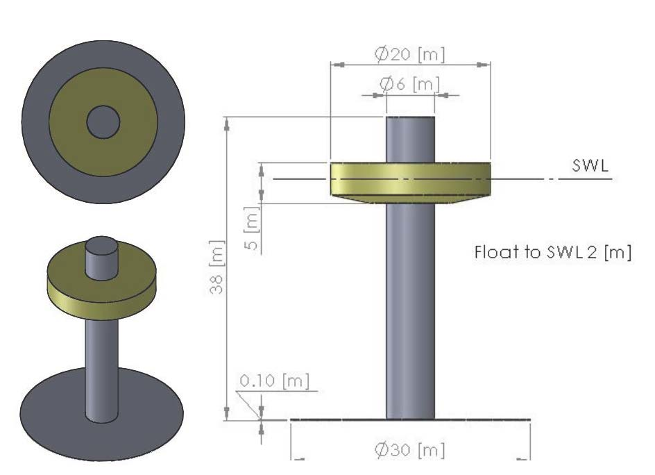
Float Full Scale Properties
CG (m)	Mass (tonne)	Moment of Inertia (kg-m^2)
0.0	727.0	20’907’301
0.0			21’306’091	4305
-0.72			4305	37’085’481

Plate Full Scale Properties
CG (m)	Mass (tonne)	Moment of Inertia (kg-m^2)
0.0	878.30	94’419’615
0.0			94’407’091	217’593
-21.29			217’593	28’542’225

Generating Hydrodynamic Data

The first step in modelling the system is to generate the hydrodynamic data files using a BEM solver such as Nemoh, WAMIT or AQUA. This will be demonstrated in this example using Nemoh. At this point it may be worth reading the section NEMOH which introduces the Matlab based preprocessor which has been developed to help with this with simple examples.

To use Nemoh, you must first generate surface meshes of the bodies you wish to simulate. Ideally these must be quadrilateral meshes, although triangular meshes can be treated as degenerate quadrilaterals. These meshes must be cut off at the mean free surface level of the water, so they will likely be different from the STL meshes used for visualisation (unless all bodies are not surface piercing). The mesh for the RM3 system for Nemoh is shown in Fig. 1 and the mesh files are provided in the geometry subdirectory. The Nemoh mesh input is defined using two files, a .nmi and a .cal file.

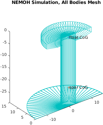
Fig. 1 Plot of both Nemoh input meshes for the RM3 example.

In this example, generating the hydrodynamic data is performed by the example_rm3.generate_hydrodata function. We will now work our way through this function to show how the process works (but remember you should first read the section NEMOH to make understanding this easier).

The start of this function just sets up from option parsing and directories etc. which aren’t important for understanding it’s actual operation:

function hydro = generate_hydrodata (varargin)

    options.PlotBEM = true;
    options.WriteH5 = true;
    options.SkipIfExisting = false;
    
    options = parse_pv_pairs (options, varargin);
    

    dir = getmfilepath ('test_wsim_RM3.generate_hydrodata');

    inputdir = fullfile (dir, 'RM3_NEMOH_output');

See the help for the parse_pv_pairs function to understand this option parsing.

The next step is to create the Nemoh body objects for the float and spar, using as input the mesh files for each:

    %% create the float

    % create a body object which will be the cylinder
    float = nemoh.body (inputdir, 'Name', 'float');

    % define the body shape using previously generated input mesh
    float.loadNemohMesherInputFile ( fullfile (dir, 'geometry', 'float.nmi'), ...
                                     fullfile (dir, 'geometry', 'float_Mesh.cal') ...
                                     ... 'CentreOfGravity', [0,0,-0.72] 
                                    );

    %% create the spar

    spar = nemoh.body (inputdir, 'Name', 'spar');

    % define the body shape using previously generated input mesh
    spar.loadNemohMesherInputFile ( fullfile (dir, 'geometry', 'spar.nmi'), ...
                                    fullfile (dir, 'geometry', 'spar_Mesh.cal') ...
                                    ... 'Draft', 28.8999996, ... % got from reading example mesh file in WEC-Sim 
                                    ... 'CentreOfGravity', [ 0, 0, -21.29 + 28.8999996 - 8.71 ] 
                                    );

The Nemoh bodies are now ready to be inserted into a Nemoh system which will process their meshes and run the Nemoh calculations.

    %% Create the nemoh simulation

    % here we insert the cylinder body at creation of the simulation, but could
    % also have done this later by calling addBody
    sim = nemoh.simulation ( inputdir, ...
                             'Bodies', [ float, spar ] );

The mesh can then be plotted, and it is this plot which was shown in Fig. 1.

    %% draw the course body mesh (this will be refined later)
    sim.drawMesh ();
    axis equal

Now the meshes can be processed. This involves writing out the Nemoh mesher input files and calling processMeshes which runs the Nemoh mesher on the the course mesh input files to produced a refined mesh, and also performs some basic hydrodynamic and geometrical calculations, with the results being put in the hydroData directory.

    % write out the course mesh files for all bodies 
    sim.writeMesherInputFiles ();

    % process mesh files for all bodies to make ready for Nemoh
    sim.processMeshes ();

    %% Draw all the now processed meshes in one figure

    sim.drawMesh ();
    axis equal;

    %% Generate the Nemoh input file

    % generate the file 
    omega = [0.02, 5.20];
    sim.writeNemoh ( 'NWaveFreqs', 260, ...
                     'MinMaxWaveFreqs', omega, ...
                     'DoIRFCalculation', false, ...
                     'NDirectionAngles', 1 );

    % The above code demonstrates the use of optional arguments to writeNemoh
    % to set the desired wave frequencies. If the wave frencies were not
    % specified a default value would be used. These are not the only possible
    % options for writeNemoh. The following optional arguments are available,
    % and the defaults used if they are not supplied are also shown:
    %
    % DoIRFCalculation = true;
    % IRFTimeStep = 0.1;
    % IRFDuration = 10;
    % NWaveFreqs = 1;
    % MinMaxWaveFreqs = [0.8, 0.8];
    % NDirectionAngles = 0;
    % MinMaxDirectionAngles = [0, 0];
    % FreeSurfacePoints = [0, 50];
    % DomainSize = [400, 400];
    % WaterDepth = 0;
    % WaveMeasurementPoint = [0, 0];
    %
    % For more information on these arguments, see the help for the writeNemoh
    % method.

    %% Run Nemoh on the input files

    sim.run ()
    

In this case we have chosen to obtain results for 260 wave frequencies. This will take quite a long time to run on a typical desktop PC or laptop, on the order of several hours, and produce several hundred MB of data in the form of text files. Generally you only want to produce these results once.

The final part of the function deals with converting the output from Nemoh into a form suitable for use in EWST.

    %% Create hydro structure for 
    
    hydro = struct();

    hydro = wsim.bemio.processnemoh (inputdir);
    
    % hydro = Read_WAMIT(hydro,'..\..\WAMIT\RM3\rm3.out',[]);
    % hydro = Combine_BEM(hydro); % Compare WAMIT
    hydro = Radiation_IRF (hydro, 60, [], [], [], 1.9);
    
    hydro = Radiation_IRF_SS (hydro, [], []);

    hydro = Excitation_IRF (hydro,157, [], [], [], 1.9);
    
    if options.WriteH5
        Write_H5 (hydro, fullfile (inputdir, 'hydroData'))
    end
    
    if options.WriteH5
        wsim.bemio.write_hydrobody_mat_files (hydro, fullfile (inputdir, 'hydroData'))
    end
    
    if options.PlotBEM
        Plot_BEMIO (hydro)
    end

end

The first step is to load the Nemo data files and convert them to a standard format. This is achieved with the wsim.bemio.processnemoh function. This function is part of a package called bemio, which is within the wsim package. Note that this is separate from the standard BEMIO functions from the original WEC-Sim project. Copies of these are provided with EWST for convenience, any new function made specifically for EWST can be found in this wsim.bemio package.

The output of wsim.bemio.processnemoh is a Matlab structure containing hydrodynamic data for all the bodies in the Nemoh system. This hydro structure can then undergo further processing as shown in the function, depending on what types of simulation are desired to be run in EWST. Here we generate the wave radiation impulse response functions for both the convolution integral calculation method and the state-space form, and also the wave excitation impulse response function.

Once all processing of the hydrodynamic data is complete, the data must be converted to a form with can be used within EWST, i.e., which can be used by the wsim.hydroBody class. This class will be discussed in more detail in the following section, but for now it is sufficient to know that the data must either be converted to on HDF5 format file, or a set of .mat files, one for each hydrodynamically interacting body. The first format is the same as used by the original WEC-Sim project. The ability to use normal .mat files directly has been added to EWST, therefore only the .h5 file can be used with both tools. Compared to the output of Nemoh, the .h5 and .mat files are quite small. The .h5 file will be on the order of tens of MB (7.4MB in this case), while the .mat files will be smaller still (two 1MB files in this case).

System Simulation

Having generated the required hydrodynamic data to calculate the wave interaction forces we are now ready to use this data in a time domain simulation of the RM3 device. The time domain simulation and system is defined in this case in one function, example_rm3.make_multibody_system and a script example_rm3.run_wecsim. Note that there is nothing special about the names of these functions, you are free to organise the code in any way you like, and name the scripts and functions any way you like.

Initial Simulation Setup

We will start by examining example_rm3.run_wecsim, which in this case is the main script which sets up and runs the simulation. The first section of this script sets the general simulation and wave parameters.

% +example_rm3/run_wecsim.m
%
% Example script demonstrating the simulation of the Reference Model 3
% buoy/spar/plate system with a basic PTO
%
%

% ensure some variables are cleared between runs (even though it's probably
% not that important)
clear waves simu hsys mbsys float_hbody spar_hbody hydro_mbnodes hydro_mbbodies hydro_mbelements lgsett wsobj

%% Hydro Simulation Data

% some global simulation settings 
simu = wsim.simSettings ( fullfile ( wecsim_rootdir(), '..', '..', 'doc', 'sphinx', 'examples', '+example_rm3'), ...
                          'Verbose', true); 
simu.startTime = 0;                   % Simulation Start Time [s]
simu.endTime=400;                     % Simulation End Time [s]
simu.dt = 0.1;                        % Simulation time-step [s]
simu.rampT = 100;                     % Wave Ramp Time Length [s]
simu.b2b = true;                      % Body-to-body interaction

%% Wave Information 

% noWaveCIC, no waves with radiation CIC  
% waves = waveClass('noWaveCIC');       %Create the Wave Variable and Specify Type      
%%%%%%%%%%%%%%%%%%%

% Regular Waves
waves = wsim.waveSettings ('regularCIC');        %Create the Wave Variable and Specify Type                               
waves.H = 2.5;                          %Wave Height [m]
waves.T = 8;                            %Wave Period [s]
%%%%%%%%%%%%%%%%%%

% Regular Waves
% waves = wsim.waveSettings ('regular');        %Create the Wave Variable and Specify Type                               
% waves.H = 2.5;                          %Wave Height [m]
% waves.T = 8;                            %Wave Period [s]
% simu.ssCalc = 1;
%%%%%%%%%%%%%%%%%%%

% Irregular Waves using PM Spectrum with Convolution Integral Calculation
% waves = wsim.waveSettings ('irregular');       %Create the Wave Variable and Specify Type
% waves.H = 2.5;                        %Significant Wave Height [m]
% waves.T = 8;                          %Peak Period [s]
% waves.spectrumType = 'PM';
%%%%%%%%%%%%%%%%%%%

% % Irregular Waves using BS Spectrum with Convolution Integral Calculation
% waves = wsim.waveSettings ('irregular');       %Create the Wave Variable and Specify Type
% waves.H = 2.5;                        %Significant Wave Height [m]
% waves.T = 8;                          %Peak Period [s]
% waves.spectrumType = 'BS';
% %%%%%%%%%%%%%%%%%%%

% Irregular Waves using BS Spectrum with State Space Calculation
% waves = wsim.waveSettings ('irregular');       %Create the Wave Variable and Specify Type
% waves.H = 2.5;                        %Significant Wave Height [m]
% waves.T = 8;                          %Peak Period [s]
% waves.spectrumType = 'BS';
% simu.ssCalc = 1;	
%Control option to use state space model 
%%%%%%%%%%%%%%%%%%%

% Irregular Waves using User-Defined Spectrum
% waves = wsim.waveSettings ('irregularImport');  %Create the Wave Variable and Specify Type
% waves.spectrumDataFile = 'ndbcBuoyData.txt';  %Name of User-Defined Spectrum File [2,:] = [omega, Sf]
%%%%%%%%%%%%%%%%%%%

% User-Defined Time-Series
% waves = wsim.waveSettings ('userDefined');     %Create the Wave Variable and Specify Type
% waves.etaDataFile = 'umpqua46229_6_2008.mat'; % Name of User-Defined Time-Series File [:,2] = [time, wave_elev]
%%%%%%%%%%%%%%%%%%%

The simulation and wave settings are each stored using classes, wsim.simSettings and wsim.waveSettings, where the settings are the class properties. Most of the settings in this example are self-explanatory, but more settings are available which may not be as obvious. A full list of the possible simulation settings and their descriptions are shown below:

Property/Setting	Description
startTime	Simulation start time (default = 0 s)
endTime	Simulation end time (default = 500 s)
dt	Simulation time step (default = 0.1 s)
dtFeNonlin	Sample time at which to calculate nonlinear forces (default = dt)
dtCITime	Sample time at which to calculate Convolution Integral (default = dt)
rampT	Ramp time for wave forcing (default = 100 s)
domainSize	Size of free surface and seabed. This variable is only used for visualization (default = 200 m)
CITime	Convolution integral time span (default = 60 s)
ssCalc	Option for convolution integral or state-space calculation: convolution integral->0, state-space->1, (default = 0)
nlHydro	Option for nonlinear hydrodynamics calculation: linear->’0’, nonlinear->’1’, (default = 0)
b2b	Option for body-to-body interactions: off->false, on->true, (default = false)
paraview	Option for writing vtp files for paraview visualization.
adjMassWeightFun	Weighting function for adjusting added mass term in the translational direction (default = 2)
mcrCaseFile	mat file that contain a list of the multiple conditions runs with given conditions
morrisonElement	Option for Morrison Element calculation: Off->’0’, On->’1’, (default = 0)
rho	Density of water (default = 1000 kg/m^3)
g	Acceleration due to gravity (default = 9.81 m/s)

For the wave settings, examples of the different types of settings are shown in the comments in this section of the script.

Creating the Hydrodynamic System

The next step is to define the system of hydrodynamically interacting bodies. This is done using the wsim.hydroBody class and the wsim.hydroSystem class. The wsim.hydroSystem class is essentially a container for a collection of hydroBody objects, with one hydroBody object for each hydrodynamic body in the system. We specifically refer to hydrodynamically interacting bodies a other bodies in the system are defined elsewhere, as part of the multibody system dynamics system. This will be explained in a later section.

The wsim.hydroBody class does all processing of the hydrodynamic forces on a body. The wsim.hydroSystem organises these bodies, inserts the correct position, velocity and acceleration information into each body, and gets all of the forces applied to the bodies by the wave action as the simulation proceeds. The motion of the system is not calculated by the hydrodynamic system, which is only concerned with the calculation of the forces.

So to define the hydrodynamic system for the RM3 example, the first step is to create two hydroBody objects:

%% Hydrodynamic body system
%
% Sets up the bodies which interact with the waves (and each other)
%
%

% Float

% Create the float_hbody object, Set the location of the hydrodynamic
% data file which must be in the case_directory/hydroData directory 
float_hbody = wsim.hydroBody('rm3.h5');
% Body Mass. The 'equilibrium' option oets it to the displaced water weight.
float_hbody.mass = 'equilibrium';                   
% Moment of Inertia matrix [kg*m^2]   
float_hbody.momOfInertia = [20907301, 21306090.66, 37085481.11];
float_hbody.geometryFile = 'float.stl';    %Location of Geomtry File

% Spar/Plate
spar_hbody = wsim.hydroBody('rm3.h5');
spar_hbody.mass = 'equilibrium';
spar_hbody.momOfInertia = [94419614.57, 94407091.24, 28542224.82];
spar_hbody.geometryFile = 'plate.stl';

% make a hydrosys object for simulation
hsys = wsim.hydroSystem (waves, simu, [float_hbody, spar_hbody]);

The hydroBody objects take as input a file name which is either .h5 file for the whole hydrodynamic system, or a .mat file specific to that body. The file is always searched for in the hydroData subdirectory of the case directory, so only the file name is required, not the full path.

Having created all the required hydroBody objects, we can put them into a hydroSystem [2] and tell it to prepare them for a time domain simulation. You must always call initialiseHydrobodies and timeDomainSimSetup before a simulation.

% make a hydrosys object for simulation
hsys = wsim.hydroSystem (waves, simu, [float_hbody, spar_hbody]);

% set up transient simulation
hsys.initialiseHydrobodies ();
hsys.timeDomainSimSetup ();

Our hydrodynamic system is now defined, and ready to be simulated, the next step is then to create the overall multibody dynamics system which constrains the motion of the bodies in the appropriate ways. The hydroSystem also takes as input the waveSettings and simSettings objects, from which it knows the location of the case directory etc.

[2]

In Matlab we can put the hydroBody objects into the hydroSystem simply by placing them in square brackets to make an array of hydroBody objects (which is what hydroSystem expects), i.e. [float_hbody, spar_hbody]. However, at the time of writing, Octave does not yet support this syntax and some small modifications are necessary. It simply requires that you instead do: obj_array(1) = float_hbody; obj_array(2) = spar_hbody; hsys = wsim.hydroSystem (waves, simu, obj_array); See the file +example_rm3/run_wecsim_in_octave.m for an example of how the run the same system in Octave. The changes are small, but important. This file also demonstrates the use of the .mat file hydroData format. This version of the file also runs in Matlab, so it is possible to create files which run under both platforms.

Creating the MultiBody System

Having set up the hydrodynamic system, the next step is to define the constraints that determine the motion of that system under the applied forces and moments. These constrained multibody system dynamics are solved by MBDyn. MBDyn is a separate program, and forces and motion are communicated between the two programs throughout the simulation via one of several available communication methods.

MBdyn normally takes as input a special data file format which defines all of the bodies and joints etc. in the system. To make the creation of systems simpler and allow systems to be completely defined using Matlab code, an advanced pre-processing tool has been developed as a part of a suite of tools in the MBDyn Matlab Toolbox, which is available as a separate standalone tool (and most likely you will have received it alongside EWST). The MBDyn Matlab Toolbox also has its own manual with simple examples demonstrating the toolbox’s capabilities. It is advisable to first examine some of the examples in this manual to get a better understanding of how the pre-processor works before attempting to develop a system for EWST, or even understand the example which is about to be described, as an in-depth discussion of the operation and organisation of MBDyn and the MBDyn preprocessor will not be repeated here.

The first step in creating the multibody system is to get the multibody elements corresponding to the hydrodynamic bodies. This task can be done automatically by wsim.hydroSystem using the makeMBDynComponents method.

%% Multibody dynamics system specification (mbdyn)

% generate the nodes and elements for simulation of the hydrodynamic system
% in MBDyn. One node and one body element are created for each hydrodynamic
% body interacting with the waves. These are then used in the larger
% multibody system with other joints, constraints and bodies
[hydro_mbnodes, hydro_mbbodies, hydro_mbelements] = hsys.makeMBDynComponents ();

This method returns three cell arrays containing the structural nodes, bodies and other elements which define the parts of the system corresponding to the hydrodynamic bodies. These components can then be linked with other components in the system. As the system requires more than a few lines of code to specify, it has been specified in a separate (heavily commented) function file in +example_rm3/make_multibody_system.m. A section of the file is shown below:

    % create a node to clamp to the global frame which we can use to attach
    % a planar joint (actually made up of two joints) to the spar. The
    % planar joint will force the spar to move in a plane attached to the
    % clamped node. This restricts the motion of the whole system to the
    % X-Z plane (this is to match the RM3 simulation from the original
    % WECSim and is not essential for any system).
    %
    % Since  we are going to clamp the node, we can make it static (getting rid
    % of the degrees of freedom associated with it)
    clamped_node = mbdyn.pre.structuralNode6dof ('static', 'AbsolutePosition', ref_seabed.pos);
    
    % clamp it with a clamp joint
    jclamp = mbdyn.pre.clamp (clamped_node, 'node', 'node');

    % apply the inPlane constraint so spar can only move in X-Z axis
    j3 = mbdyn.pre.inPlane (  clamped_node, spar_node, [0;1;0], ...
                              'RelativeOffset', 'null', ...
                              'RelativeOffsetReference', 'other node');
                          
    % add a prismatic joint (keeps the orientation of two nodes fixed, i.e.
    % they won't rotate relative to each other)
    j1 = mbdyn.pre.prismatic (float_node, spar_node);

    
    % The next section creates the pto mechanism constraints
    
    % create an orientation which points along the global Z axis 
    om = mbdyn.pre.orientmat ( '2vectors', ...
                               struct ( 'ia', 1, ...
                                        'vecA', [1., 0., 0.], ...
                                        'ib', 3, ...
                                        'vecB', [0., 0., 1.] ) ...
                             );
                           
	% restrain the two nodes to both move along a line attached to the
	% first node which is initially parallel to the Z axis
    j2 = mbdyn.pre.inline ( float_node, spar_node, ...
                            'RelativeLinePosition', [0;0;0], ...
                            'RelativeOrientation', om, ...
                            'OrientationReference', 'global' );


	% create an orientation with axis 3 pointing along the global axis 2

The full system requires the creation of five joint elements and another node to act as a reference so the motion can be restricted to being only in the X-Z plane. This function assembles all of the multibody dynamics elements into a mbdyn.pre.system object which organises and controls them in a similar way to the wsim.hydroSystem class.

    % assemble the system
    mbsys = mbdyn.pre.system ( prob, ...
                               'Nodes', [hydro_mbnodes, {clamped_node}], ...
                               'Elements', [{float_mb_body, spar_mb_body, jclamp, j1, j2, j3, j4 socket_force}, hydro_mbelements], ...
                               'DefaultOrientation', 'orientation matrix', ...
                               'DefaultOutput', problem_options.DefaultElementOutput );
                           

In the run_wecsim script, it is this system with is returned by the call to example_rm3.make_multibody_system. The resulting system can be plotted in a figure:

% draw it in a figure
mbsys.draw ( 'Mode', 'ghost', ...
             'Light', true, ...
             'AxLims', [-30, 30; -30, 30; -35, 35], ...
             'Joints', false, ...
             'StructuralNodes', true);

The result of the call to draw above is shown in Fig. 2

Many options are possible with the draw option, for example, a prettier output (but less useful for checking the locations of nodes etc.) can be produced with the ‘solid’ mode:

mbsys.draw ( 'Mode', 'solid', ...
             'Light', true, ...
             'AxLims', [-30, 30; -30, 30; -35, 35], ...
             'Joints', false, ...
             'StructuralNodes', false);

The result of this is shown in Fig. 3

Adding a Power Take-Off

The next step is to add a power take-off to the simulation. For this example we want to add simple damper, i.e. a force which is linearly related to the relative velocity of the two parts of the RM3 device. We will calculate this force in Matlab, base on the motion of the WEC, and send it to MBDyn during the simulation. To implement this, it is necessary to first get the motion in 3D space of float and spar and determine their relative velocity in a direction parallel to the orientation of the spar. Then the damping force must be calculated, and converted to a 3D force vector to be applied to the nodes attached to each body in MBDyn.

EWST makes the process of calculating and applying power take-off forces easy by providing a set of power take-off classes (for different types of motion) which perform most of this work, leaving only the calculation of scalar force value to the user. These classes are the wsim.linearPowerTakeOff and wsim.rotaryPowerTakeOff classes, and their main function is to automate getting the correct nodal motion from MBDyn during the simulation, and from this motion determine the relative velocity and position of two components in a simulation (or the relative angular velocity and position in the case of wsim.rotaryPowerTakeOff), and then calculate the force vector on the nodes. Both of these classes come with extensive help which can be accessed using the normal Matlab help systems, e.g. run

doc wsim.linearPowerTakeOff

to open the help for this class in the help browser, or

help wsim.linearPowerTakeOff

to view text help in the command line. See The Matlab Help System for more information on the Matlab and Octave help systems.

For this RM3 example we will use the wsim.linearPowerTakeOff class. This class allows you to apply a force which is calculated by a function with the syntax:

force = force_function (time, displacement, velocity)

You are free to create and use any Matlab function with this syntax as the calculation of the power take-off force. For the RM3 example, the supplied function is a spring-damper function, although in this case, the spring constant is set to zero. In the example, the function is defined in the body of the script as an anonymous function, but it can also be any other function on the Matlab path. In this case the function accepts the time variable as an input, but just ignores it.

%% Set up Power Take-Off (PTO)

% set up a simple linear spring-damper power take-off force based on a
% matlab function. See help for
k = 0;
c = 1200000;

forcefcn = @(time, xRpto, vRpto) -k*xRpto -c*vRpto;

% create a power take-off object attached to the two hydro nodes, with the
% force being based on the relative velocity and displacement along axis 3
% of the first (reference) node (in it's coordinate frame).
pto = wsim.linearPowerTakeOff ( hydro_mbnodes{2}, hydro_mbnodes{1}, 3, forcefcn );

It can be seen that setting up of the PTO is made very simple by wsim.linearPowerTakeOff. It simply requires the two nodes attached to each part of the PTO, an axis number, and the force function. The PTO class then does all the work of applying the correct forces to the nodes. The PTO calculates the forces based on the relative displacement and velocity of the two nodes in a direction parallel to the specified axis number in the reference frame of the first node.

Running the Simulation

With all of the possible components describing the system now assembled it would now be possible to start manually stepping through the system, and indeed this is possible (in case total control is needed). However, to make running and managing the simulation easy, the wsim.wecSim class has been provided. This class takes in all the previously define components and runs the simulation. One of the most useful aspects of wsim.wecSim is that is ensures the correct hydrodynamic and PTO force are applied to the correct nodes. The wsim.wecSim class also does extensive logging of simulation data for examination afterwards. This logging is also highly configurable so it can be selectively deactivated to improve simulation speed. [3]. The logging during a simulation is performed by another class, the wsim.logger class. A logger object is created inside wsim.wecSim and returned at the end of a simulation. The settings controlling the logging, are themselves contained in another class, wsim.loggingSettings. It is the loggingSettings class which is created next in the example script.

[3]

Logging of data usually requires some reallocation of memory. The wsim.logger class used in EWST attempts to do this in an efficient way (one can preallocate the size of the memory required to log the data, and memory is automatically grown in blocks when the preallocated limit is reached). However, the time spent doing this is still non-negligible. If efficiency is crucial, e.g. within an optimisation procedure, one should only log what is really necessary for optimum simulation speed.

%% Run the simulation

lgsett = wsim.loggingSettings ();

lgsett.positions = true;
lgsett.velocities = true;
lgsett.accelerations = true;
lgsett.nodeForces = true;
lgsett.nodeForcesUncorrected = true;
lgsett.forceHydro = true;
lgsett.forceExcitation = true;
lgsett.forceExcitationRamp = true;
lgsett.forceExcitationLin = true;
lgsett.forceExcitationNonLin = true;
lgsett.forceRadiationDamping = true;
lgsett.forceRestoring = true;
lgsett.forceMorrison = true;
lgsett.forceViscousDamping = true;
% lssett.ForceAddedMassUncorrected = false;
lgsett.momentAddedMass = true;
lgsett.nodeMoments = true;
lgsett.nodeMomentsUncorrected = true;
lgsett.momentHydro = true;
lgsett.momentExcitation = true;
lgsett.momentExcitationRamp = true;
lgsett.momentExcitationLin = true;
lgsett.momentExcitationNonLin = true;
lgsett.momentRadiationDamping = true;
lgsett.momentRestoring = true;
lgsett.momentMorrison = true;
lgsett.momentViscousDamping = true;
% lssett.momentAddedMassUncorrected = false;
lgsett.momentAddedMass = true;

lgsett.forceIterations = true;
        

It can be seen that there is quite fine grained control over what is logged. It is not necessary to set every setting as shown in the script, this is just provided to demonstrate what settings are available. By default, all logging is active (everything will be logged). One can then selectively deactivate components by setting them to false. Alternatively, the loggingSettings class has a method allOff, which deactivates all logging (sets all logging settings to false). One can then selectively reactivate only those variables which are to be logged during the simulation by setting them to true [4].

Having chosen the desired logging settings, the simulation is ready to be run. The next step is then to create the wsim.wecSim object discussed previously.

% create the wecSim object
wsobj = wsim.wecSim ( hsys, mbsys, ...
                      'PTO', pto, ... % multiple PTOs may be added
                      'LoggingSettings', lgsett );

The wsim.wecSim object must take as input the wsim.hydroSystem and mbdyn.pre.system objects on creation. The supply of one or more PTO objects is optional (and they can also be added later using the addPTO method), as is the supply of a wsim.loggingSettings object. If no loggingSettings onject is supplied, one is created internally by wsim.wecSim with all default settings, so everything will be logged. See the help for wsim.wecSim for more detail on how to create the object and what options are available.

Having created the wecSim management object we can then prepare and run the simulation. The prepare method must always be called before a simulation can be run.

% initialise the simulation
wsobj.prepare ();

% run it and get the output data. The results from wecSim are stored in a
% wsim.logger object. What's stored in here is controlled by the
% loggingsettings above, but also by each PTO object, which controls its
% own logging output. 
[datalog, mbdyn_pproc] = wsobj.run ('TimeExecution', true);

The run method then does several things. It creates an input file for MBDyn and writes it to disk [5], it then launches the MBDyn program and sets up communication with it, and it then steps though the simulation and returns two outputs. The first output is the wsim.logger object discussed previously which contains the logged data from the simulation. The second output is an object of the class mbdyn.postproc. Both of these outputs will be discussed in more detail in the next section.

There are many options available for the run method which are documented in it’s help. In this case we used only one, the 'TimeExecution' option, which prints the wall-clock time taken to perform the simulation.

[4]	It should also be noted that setting some logging settings to true indirectly causes some other variables to also be logged. For example, setting forceAddedMass to true will also cause forceAddedMassUncorrected to become true as this is required to calculate the final added mass force.

[5]	By default these files are written to a subdirectory of the case directory named output_<date_and_time> where <date_and_time> is replaced by the date and time the run method was started. The output from MBDyn is also placed in this directory.

Examining The Results

Having run the simulation, it is now possible to use the returned wsim.logger object and mbdyn.postproc object to examine what occurred during the simulation. The wsim.logger object generally contains data which was created on the Matlab side of the simulation, i.e. the hydrodynamic and PTO forces, but also data which was sent by MBDyn during the simulation such as node positions etc. The mbdyn.postproc method in contrast can be used to access other more detailed data calculated by MBDyn during the simulation and written to disk once the simulation was complete. This includes data on all the internally calculated forces etc.

The data in wsim.logger object is stored in a public property, data, which is a Matlab structure with field names corresponding to each logged data item. For example, the contents of data in the datalog output of the RM3 example is the following:

>> datalog.data

ans =

  struct with fields:

                          Time: [4001×1 double]
                     Positions: [3×2×4001 double]
              AngularPositions: [3×2×4001 double]
                    Velocities: [3×2×4001 double]
             AngularVelocities: [3×2×4001 double]
                 Accelerations: [3×2×4001 double]
          AngularAccelerations: [3×2×4001 double]
                    NodeForces: [3×2×4001 double]
         NodeForcesUncorrected: [3×2×4001 double]
                    ForceHydro: [3×2×4001 double]
               ForceExcitation: [3×2×4001 double]
           ForceExcitationRamp: [3×2×4001 double]
            ForceExcitationLin: [3×2×4001 double]
         ForceExcitationNonLin: [3×2×4001 double]
         ForceRadiationDamping: [3×2×4001 double]
                ForceRestoring: [3×2×4001 double]
                 ForceMorrison: [3×2×4001 double]
           ForceViscousDamping: [3×2×4001 double]
                ForceAddedMass: [3×2×4001 double]
     ForceAddedMassUncorrected: [3×2×4001 double]
                   NodeMoments: [3×2×4001 double]
        NodeMomentsUncorrected: [3×2×4001 double]
                   MomentHydro: [3×2×4001 double]
              MomentExcitation: [3×2×4001 double]
          MomentExcitationRamp: [3×2×4001 double]
           MomentExcitationLin: [3×2×4001 double]
        MomentExcitationNonLin: [3×2×4001 double]
        MomentRadiationDamping: [3×2×4001 double]
               MomentRestoring: [3×2×4001 double]
                MomentMorrison: [3×2×4001 double]
          MomentViscousDamping: [3×2×4001 double]
               MomentAddedMass: [3×2×4001 double]
    MomentAddedMassUncorrected: [3×2×4001 double]
           PTO_1_InternalForce: [4001×1 double]
    PTO_1_RelativeDisplacement: [4001×1 double]
        PTO_1_RelativeVelocity: [4001×1 double]

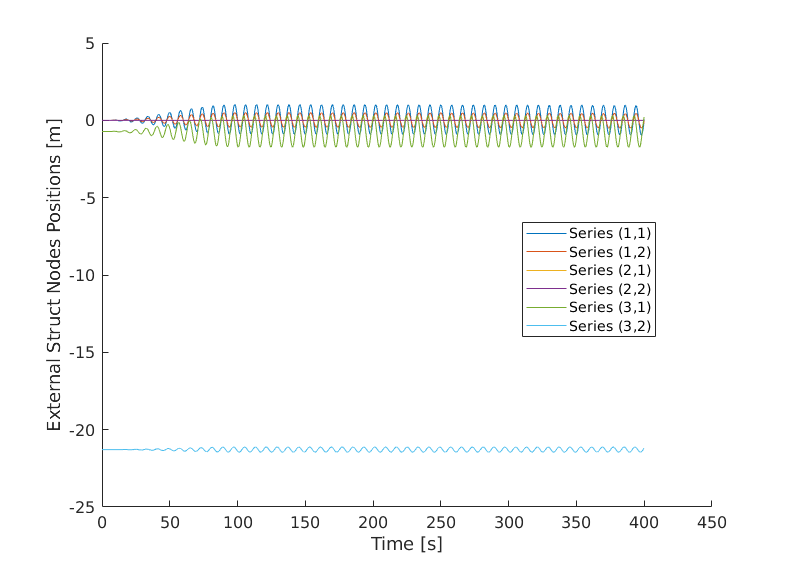
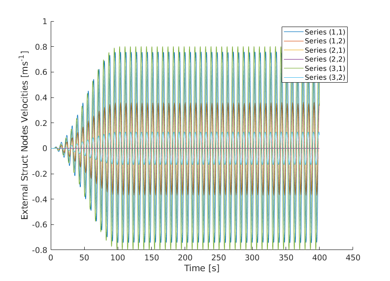
This can be accessed an processed or plotted like any normal Matlab variable. However, for convenience, the wsim.logger class provides methods to plot the outputs directly. The main method for this is plotVar. The plotVar method is called with the name of the variable to be plotted and plots it against it’s independent variable, which in most cases is the Time variable. This is shown for several variables in the example:

%% Plot some results

datalog.plotVar ('Positions');

datalog.plotVar ('Velocities');

% plot the force from the PTO (note the 'PTO_1_' prefix added by
% wsim.wecSim, this allows multiple PTO objects of the same type to by
% used in one system)
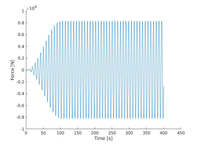
datalog.plotVar ('PTO_1_InternalForce');

The plots produced by these calls to plotVar are shown in Fig. 4, Fig. 5 and Fig. 6.

The log returned by the wecSim object only contains motion data for the nodes which are accessed through the external structural force, there may be other nodes in the simulation, and data on the other nodes in the simulation must be obtained from the output of MBDyn. As mentioned previously, the second output of the run method, is the mbdyn.postproc object. This object loads data from a netcdf format data file produced by MBDyn at the end of the simulation. A list of all the variables which can then be examined using this object is produced using the displayNetCDFVarNames method, e.g. for the RM3 example, this produces the following:

>> mbdyn_pproc.displayNetCDFVarNames ()
run.step : time step index
time : simulation time
run.timestep : integration time step
node.struct : Structural nodes labels
node.struct.1 : no description
node.struct.1.X : global position vector (X, Y, Z)
node.struct.1.R : global orientation matrix (R11, R21, R31, R12, R22, R32, R13, R23, R33)
node.struct.1.XP : global velocity vector (v_X, v_Y, v_Z)
node.struct.1.Omega : global angular velocity vector (omega_X, omega_Y, omega_Z)
node.struct.2 : no description
node.struct.2.X : global position vector (X, Y, Z)
node.struct.2.R : global orientation matrix (R11, R21, R31, R12, R22, R32, R13, R23, R33)
node.struct.2.XP : global velocity vector (v_X, v_Y, v_Z)
node.struct.2.Omega : global angular velocity vector (omega_X, omega_Y, omega_Z)
node.struct.3 : no description
node.struct.3.X : global position vector (X, Y, Z)
node.struct.3.R : global orientation matrix (R11, R21, R31, R12, R22, R32, R13, R23, R33)
node.struct.3.XP : global velocity vector (v_X, v_Y, v_Z)
node.struct.3.Omega : global angular velocity vector (omega_X, omega_Y, omega_Z)
elem.autostruct : AutomaticStructural elements labels
elem.joint : Joint elements labels
elem.force : Force elements labels
node.struct.1.B : momentum (X, Y, Z)
node.struct.1.G : momenta moment (X, Y, Z)
node.struct.1.BP : momentum derivative (X, Y, Z)
node.struct.1.GP : momenta moment derivative (X, Y, Z)
node.struct.2.B : momentum (X, Y, Z)
node.struct.2.G : momenta moment (X, Y, Z)
node.struct.2.BP : momentum derivative (X, Y, Z)
node.struct.2.GP : momenta moment derivative (X, Y, Z)
elem.joint.7 : no description
elem.joint.7.f : local reaction force (Fx, Fy, Fz)
elem.joint.7.m : local reaction moment (Mx, My, Mz)
elem.joint.7.F : global reaction force (FX, FY, FZ)
elem.joint.7.M : global reaction moment (MX, MY, MZ)
elem.joint.8 : no description
elem.joint.8.f : local reaction force (Fx, Fy, Fz)
elem.joint.8.m : local reaction moment (Mx, My, Mz)
elem.joint.8.F : global reaction force (FX, FY, FZ)
elem.joint.8.M : global reaction moment (MX, MY, MZ)
elem.joint.10 : no description
elem.joint.10.f : local reaction force (Fx, Fy, Fz)
elem.joint.10.m : local reaction moment (Mx, My, Mz)
elem.joint.10.F : global reaction force (FX, FY, FZ)
elem.joint.10.M : global reaction moment (MX, MY, MZ)
elem.joint.10.R : global orientation matrix (R11, R21, R31, R12, R22, R32, R13, R23, R33)
elem.joint.10.Omega : local relative angular velocity (x, y, z)

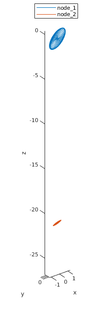
This shows the list of available variables and a short description of each. The contents of these can then be accessed using the getNetCDFVariable method. When it is created, the mbdyn.postproc class also immediately loads the motion data from the MBDyn output file for all the nodes in the simulation. Some methods for plotting this motion data are then provided, such as the plotNodeTrajectories method demonstrated in the script:

%% Plot some results

datalog.plotVar ('Positions');

datalog.plotVar ('Velocities');

% plot the force from the PTO (note the 'PTO_1_' prefix added by
% wsim.wecSim, this allows multiple PTO objects of the same type to by
% used in one system)
datalog.plotVar ('PTO_1_InternalForce');

The output of this command is shown in Fig. 7. As usual you can learn about the full range of post-processing methods available from the mbdyn.postproc object by examining the help for the class, but also through the documentation for the Matlab NBDyn Toolbox.

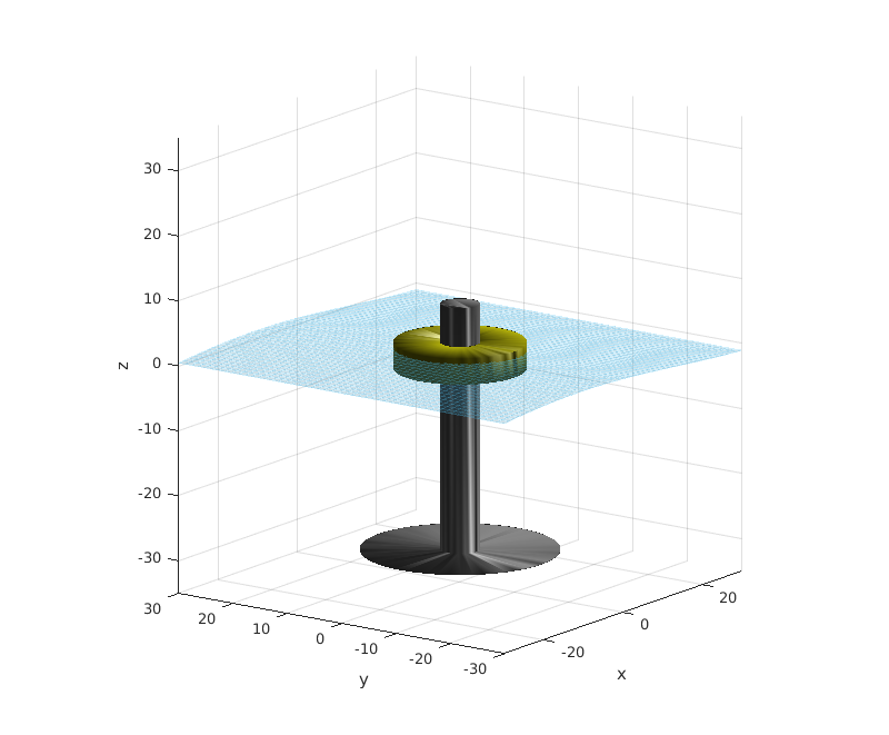
Finally, it can also be extremely helpful to visualise the motion of the system during the simulation. This can be done using the animate method of the wsim.wecSim class. An example of this is shown at the end of the script.

%% Animate the system

% create an animation of the simulation
wsobj.animate ( 'DrawMode', 'solid', ...
                'Light', true, ...
                'AxLims', [-30, 30; -30, 30; -35, 35], ...
                'DrawNodes', false, ...
                'View', [-53.9000e+000, 14.8000e+000], ...
                'FigPositionAndSize', [200, 200, 800, 800] );
             
             

A still image from the resulting animation is shown in Fig. 8. It can be seen that the wave surface is plotted in addition to the device. This animation by defuat is just played in a Matlab figure window, however, if desired, it can also be written to disk as an avi file. See the help for the wsim.wecSim.animate for more information.

Conclusions

This example gives a good introduction to the capabilities of EWST, but is not exhaustive. Topics which of interest which have not been explored include multi-rate simulation techniques, creating your own power take-off classes derived from the built-in power take-off classes, and advanced features of MBDyn that may be useful for system simulation.

Note also that further examples are provided in the same location as the example described in this document.